Lecture 05 - Noise

Noise

We like randomness because it adds complexity and surprise into our work

We have already talked about some of the issues with using randomness directly. Randomness is too chaotic for many purposes.

There are a number of processes that seem random, but they aren’t completely random – there is a correlation between events

For example, the ridge line of a mountain is random, but any particular point is influenced by the points on either side of it

Strictly speaking, we have to acknowledge that nothing in nature is truly random – they are complex

The ridge line was formed by tectonic pressures and erosion from the weather

So, many times when we reach for randomness, we are really looking for a shortcut to approximate a complex system of forces

The problem comes because pure randomness isn’t the best model Natural phenomenon have coherence on a local level

We have seen one approach to this, thinking in terms of small amounts of random variance from a pervious value

Another approach would be to use a statistical model, like a Markov chain

The solution we are going to talk about today is noise

Original and most popular form of noise is Perlin noise, created by Ken Perlin (he developed it for Tron). Incidentally, the academy decided Tron was ineligible for an effects award because it used computers, which was considered “cheating”. Perlin later won a lifetime achievement award for his work.

Like our pseudorandom number generators, a noise function returns values between 0 and 1

It works by generating random numbers at fixed points in the domain and then processing the values to create a continuous function across the entire domain

Because of this, the results of calling noise are stable while the sketch is being run. If we call noise with a particular input, we will always get the same result back.

We know that behind the scenes, our random number generator is really just spitting out numbers in a sequence. Imagine we could access that sequence at any point – to look between the numbers it spat out.

Generating noise

We can start by looking at a graph of random values. This is also a good moment to look more closely at our inadequate random function we developed earlier

Random and noise grapher sketch

Our fake random sequence has some obvious glitches – why?

We are going to use our fake random generator now, just because we have the ability to enter in values

Simple version

For values in between the integers, we do linear interpolation

const noise1 = (i) =>{
    const f = i % 1;
    const x = Math.floor(i);
    return lerp(fakeRandom(x), fakeRandom(x+1), f);
}

using the grapher, we can see the difference – we went from chaos to a coherent line

It has to be admitted, however, that the spikes are unaesthetic. This is caused by our doing linear interpolation between the points.

Advanced version

We can make a curve that goes through the points

We can do this by varying the parameter we pass to the interpolator so it isn’t linear

We are using polynomials to create the curve. These create an ease curve that smooths out the transitions.

We can use a Hermite interpolation \(3f^2 + 2f^3\)

const noise2 = (i) =>{
    const f = i % 1;
    const u = (3 - 2 * f)*f*f // Hermite interpolation "smoothstep"
    const x = Math.floor(i);
    return lerp(fakeRandom(x), fakeRandom(x+1), u);
}

Or we could use Perlin’s equation \(6f^5 - 15f^4 + 10f^3\)

const noise3 = (i) =>{
  const f = i % 1;
  
  const u = ((6 * f - 15)* f + 10) * f * f * f; // Perlin smooth step
  const x = Math.floor(i);

  return lerp(fakeRandom(x), fakeRandom(x+1), u);
}

Multi-dimensional noise

Noise functions are frequently used to create textures, so we need them to work in multiple dimensions

To get 2D noise, imagine we have a grid of random numbers and we are interpolating from one point to another. Again, we don’t use liner interpolation, we will use a cubic so that we get smooth interpolation.

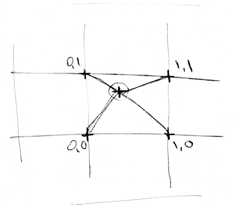(from The book of Shaders) If we graph the noise values as height, we can think of a shape like this

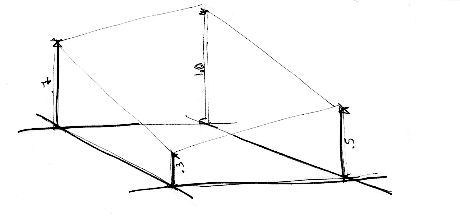(from The book of Shaders)

With our easing curve, then we get a shape like this:

(from The book of Shaders)

Getting our noise value for a particular x,y coordinate is, in essence, just sampling this surface and getting its height at that location.

To get 3D noise, we will do the same, but we will be interpolating between the eight points of a unit cube

This approach gives us something called value noise. We get a better effect with gradient noise, which interpolates gradients (basically direction vectors) instead of values. Perlin’s algorithm uses gradient noise – value noise is just easier to explain and we just want the general idea.

p5.js noise

`noise(x,y,z)

We can use this like random() to generate values between 0 and 1. it can take 1, 2, or 3, inputs (1D, 2D, or 3D noise). Note that in all cases it returns a single value. The dimensionality just refers to the dimensions we would like to have coherence across. We frequently will think of the inputs as referring to either spatial dimensions or time.

noiseSeed()

Just like randomSeed(), we use this to have repeatable values.

noiseDetail(lod, falloff)

We can get more interesting noise by combining together noise at different scales (or frequencies). We call these octaves . The lod tells the algorithm how many octaves to combine together. The more octaves, the more detailed our noise will be, with a corresponding increase in run time).

The falloff tells us how to combine these octaves together. Valid numbers are between 0 and 1, and this sets the level of contribution of each successive octave. For example, setting this to 0.5 means that each octave will contribute 50% of the amount contributed by its predecessor. Setting this to more than .5 can mean that our noise values can be larger than 1.

Examples

1D noise We can start by looking at a representative of the output of the noise

I added a feature that allows us to drag the line along to see how the pattern continues

It isn’t much to look at at this scale – it just looks random.

As we zoom in, we can see that we are getting more and more local, creating smoother transitions

1D noise example

2D noise field

This is just a collection of rectangles colored using the noise function. Basically I am just plugging in the x, y coordinates to noise() and using the result to generate a luminance value instead of an offset.

Oddly, at this scale we can see it repeat. This is because Perlin noise expects the input coordinates to be in \([0, 256]\). Fortunately, we can zoom in between these points as much as we want, so we won’t see this effect often.

Again, as we zoom in, we can see that we are getting more and more local, creating smoother transitions

2D noise example

Clouds It doesn’t take much to take this noise field to make clouds

clouds example

Lava Changing the colors around and we can make some lava

Lava example

Fabric One of my favorite effects is making fabric like textures

Here we just have a collection of horizontal lines that we make by making small steps with x across the page. At each point we consult the noise function with the x and y value and then permute the y position by the noise

To get the movement, we take advantage of the third argument I tend to think of this as a stack of 2D noise fields. We can move up and down between the fields, and there will be a coherence between the different levels, which gives us the relatively smooth animation

Fabric example

Terrain generation Terrain generation is a place where we see a lot of the use of Perlin noise

Note that this isn’t 3D noise – it is 2D noise. We are using the x and y coordinates to generate a noise value, and we use the noise value as the height. A place where we might properly use the 3D noise in a 3D space would be to create a three dimensional texture for something like wood or marble. Instead of generating a texture that is like a decal that is wrapped around the shape, we can sample the 3D noise space.

Terrain example