Entanglement and CHSH

1 Learning Goals

Describe entangled states and product states
Describe why entanglement helps us win a game
Determine if a 2-qubit state is entangled
Analyze 2 qubit systems

2 CHSH Game Set-Up

The CHSH Game is a game played between two players (we’ll call them Amir and Bei) and a referee. The two players can strategize before the start of the game, but once the game starts, they are not allowed to communicate.

The referee sends Amir a bit $x$ and Bei a bit $y$. Then Amir must respond by sending a bit $a$ back to the referee, and likewise Bei responds by sending a bit $b$ back to the referee. Amir and Bei win the game if

when $xy=00, 01,$ or $10$, they return $a$ and $b$ such that $a=b$ (so $ab=00$ or $11$)
when $xy=11$, they return $a$ and $b$ such that $a\neq b$ (so $ab=10$ or $01$)

We can succinctly represent this relationship as wanting \[a\oplus b = x\wedge y,\] where $\oplus$ means addition modulo 2, and $\wedge$ is Boolean AND.

On your problem set, you will argue that there is a strategy (without using quantum) that allows Amir and Bei to win $75\%$ of the time. It turns out this is the best Amir and Bei can do classically

Now suppose we give Amir and Bei each a qubit. They are still not allowed to communicate once the game starts.

So far we have been thinking of qubits as photons, but in this case, we will use diamond nitrogen vacancy centers or NV centers. The key properties of NV centers are that (unlike photons) they don’t move around, they just sit at a particular place in a diamon, and the qubits they form are very stable, lasting ~1sec before decohering.

Note

(A bit of physics/materials science - feel free to read if interested.) An NV center is a created from small piece of manufactured diamond. A diamond is a lattice is made of carbon atoms, but in an NV center there is a defect where a carbon atom gets replaces by a nitrogen atom. This defect allows for relatively stable electronic states: one with a single unpaired electron, and one with two paired electrons, forming our $\ket{0}$ and $\ket{1}$ states. When there are two paired electrons, it causes photoluminscence when a light is shined on the diamond, but there is no photoluminescence with the single electron. In this way, we can make the measurement $M=\{\ket{0},\ket{1}\}.$

ABCD Question

If Amir’s qubit is in the state $\ket{0}$, and Bei’s qubit is in the state $\ket{1}$, how do we represent the combined state of both qubits?

$\ket{0}\otimes\ket{1}$
$\ket{0}_A\ket{1}_B$
$\ket{01}_{AB}$
$\ket{01}$

The $\otimes$ is read as “tensor product” or “tensor” and mathematically denotes the Kronecker product. The subscripts $A$ and $B$ are for clarity and can be dropped if the order is clear. Note that when a bra is followed by a ket, they collapse to form a number, but when a ket is followed by a ket, you just get a bigger ket.

2.1 Generic 2-qubit state

Any two-qubit state can be written in the following form (and anything written in the following form represents a two-qubit state):

\[\ket{\psi}_{AB}=a_{00}\ket{00}_{AB}+a_{01}\ket{01}_{AB}+a_{10}\ket{10}_{AB}+a_{11}\ket{11}_{AB},\quad \textrm{s.t. }a_i\in \mathbb{C}, \textrm{ and } \sum_{i\in \{0,1\}^2}|a_i|^2=1,\] where again we call $a_{00},a_{01},a_{10},a_{11}$ amplitudes.

Within each ket, the first $0$ or $1$ represent the A qubit and the second $0$ or $1$ represents the $B$ qubit. The subscripts after each ket help us keep track of this fact. However, we will frequently drop these subscripts once we have initially established that the first qubit is $A$ and the second is $B$.

Vector Note

A two qubit state can be represented as a vector in $\mathbb{C}^4$. To do this we write: \[\ket{\psi}=\left( \begin{array}{c} a_{00}\\ a_{01}\\ a_{10}\\ a_{11} \end{array}\right) \] with the amplitudes as the elements of the vector.

2.2 CHSH Strategy

Before the start of the game, Amir and Bei get together to strategize, and as part of their strategizing, they decide to share a two-qubit state, where Amir has the $A$ qubit and Bei has the $B$ qubit: \[\ket{\psi}_{AB}=\frac{1}{\sqrt{2}}\left(\ket{00}+\ket{11}\right)=\frac{1}{\sqrt{2}}\ket{00}+\frac{1}{\sqrt{2}}\ket{11}.\]

Note that \[\left|\frac{1}{\sqrt{2}} \right|^2+\left|\frac{1}{\sqrt{2}} \right|^2=1\] so this is a properly normalized state.

2.3 Winning the CHSH Game

The state $\frac{1}{\sqrt{2}}\ket{00}+\frac{1}{\sqrt{2}}\ket{11}$ has a very special correlation between the $A$ and $B$ qubits, which we call entanglement.

This correlation shows up when you make measurements. If we think of these two qubits as photons, and you take two linear polarizing filters both at the same angle, and pass each photon through one of these filters, either both photons will pass through the filters (and both collapse to have the same polarization as the filters), or both photons will be blocked. Thus the measurement outcomes are perfectly correlated. Importantly, this perfect correlation occurs no matter what the angle of the filters is.

If one polarizing filter is at a $\pi/2=90^\circ$ angle to the other filter, one photon will always pass through and one will be blocked. The again occurs for any angle of linear polarizing filters, as long as their relative angle is $\pi/2$. Thus the measurements are perfectly anticorrelated.

However, if we have two polarizing filers that are not at exactly the same angle, and are instead at a relative angle of $\pi/8$, then the measurements will be correlated with probability $\approx 0.85$. Likewise, if we have two polarizing filters that are not at exactly a $\pi/2$ angle relative to each other, but are instead at $\pi/2\pm \pi/8$, the results of the measurements will be anticorrelated with probability $\approx 0.85$.

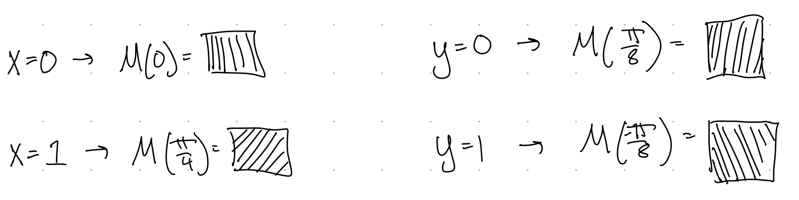
Given this, consider the following strategy for Alice and Bob, assuming they start with the state $\frac{1}{\sqrt{2}}\ket{00}+\frac{1}{\sqrt{2}}\ket{11}$. (In reality, their measurements would not look like polarizing filters, because they actually have diamonds rather than photons, but it is much easier to understand what is going on if we think about this visually in terms of angles!)

Questions from referees and the corresponding measurements Amir and Bei choose to use in the CHSH strategy, represented as polarizing filters

Group Exercise

What is Amir and Bei’s success strategy in the CHSH game with this strategy and why?

3 Entanglement

3.1 Definitions

How did the quantum state help us win the CHSH game? The state \[\frac{1}{\sqrt{2}}\ket{00}_{AB}+\frac{1}{\sqrt{2}}\ket{11}_{AB}\] has a special property: entanglement.

Definition 1

A state $\ket{\psi}_{AB}$ is a product state if $\exists \ket{\psi_1},\ket{\psi_2}$ such that $\ket{\psi}_{AB}=\ket{\psi_1}_A\ket{\psi_2}_B$.
A state $\ket{\psi}_{AB}$ is an entangled state if $\neg\exists \ket{\psi_1},\ket{\psi_2}$ such that $\ket{\psi}_{AB}=\ket{\psi_1}_A\ket{\psi_2}_B$.

In other words, there are valid $2$-qubit states that can not be described as $A$ system in one state and $B$ system in another state, but rather, the $A$ system and the $B$ system are correlated.

This is similar to classical correlation. An example of classical correlation is if you have two bits, and the probability that both bits have value $0$ is $1/2$, and the probability that both bits have value $1$ is $1/2$. If you ask what value the first bit has, I don’t know, but I do know that there is a relationship between the two bits.

3.2 Determining Whether a State is Entangled

Suppose we have two qubits in the following generic individual states

Qubit A: $\ket{\psi_1}_A=a_0\ket{0}+a_1\ket{1}$
Qubit B: $\ket{\psi_2}_B=b_0\ket{0}+b_1\ket{1}$

Then their combined state can be written as \[ \begin{align} \ket{\psi}_{AB}=&\ket{\psi_1}_A\otimes \ket{\psi_2}_B& \textrm{stick kets together with }\otimes\textrm{ to combine}\\ =&\ket{\psi_1}_A \ket{\psi_2}_B & \textrm{ $\otimes$ is optional}\\ =&(a_0\ket{0}+a_1\ket{1})_A(b_0\ket{0}+b_1\ket{1})_B&\textrm{substituting single qubit states}\\ =&a_0b_0\ket{0}_A\ket{0}_B+a_0b_1\ket{0}_A\ket{1}_B+a_1b_0\ket{1}_A\ket{0}_B+a_1b_1\ket{1}_A\ket{1}_B&\textrm{Distribute the (hidden) }\otimes\textrm{ product}\\ =&a_0b_0\ket{00}+a_0b_1\ket{01}+a_1b_0\ket{10}+a_1b_1\ket{11}&\textrm{combine the double ket into a single ket with two bits}\\ \end{align} \]

On the other hand, general 2-qubit states do not have this product structure to their amplitudes, and are written as \[\ket{\psi}_{AB}=a_{00}\ket{00}+a_{01}\ket{01}+a_{10}\ket{10}+a_{11}\ket{11},\quad \textrm{s.t. }a_i\in \mathbb{C}, \textrm{ and } \sum_{i\in \{0,1\}^2}|a_i|^2=1.\]

To prove that a state is entangled, we will use a proof by contradiction:

Group Exercise

[QI3]

Prove \[\frac{1}{\sqrt{2}}\ket{00}_{AB}+\frac{1}{\sqrt{2}}\ket{11}_{AB}\] is entangled

Proof. Assume for contradiction that $\ket{\beta_{00}}_{AB}$ is not entangled. Then it can be written in the form of a product state. Show that you get a contradiction when you try to do this.

4 Analyzing Two Qubit Product Measurements

In the CHSH game, we had the situation of having two qubits, and making individual single-qubit measurements on each qubit. We saw that for certain entangled states, these measurements could be correlated in strange ways. Now we will learn how to formally make these types of measurements and determine the probabilities of the possible outcomes.

Let the initial state of the two qubits be $\ket{\psi}_{AB}$. If the measurement on qubit $A$ is $M_{A}=\{\ket{\alpha_{0}},\ket{\alpha_{1}}\}$, and the measurement on qubit $B$ is is $M_{B}=\{\ket{\beta_{0}},\ket{\beta_{1}}\}$, there are multiple possible combinations of possible measurement outcomes. For example, the measurement on qubit $A$ could result in outcome $\ket{\alpha_{1}}$, and the measurement on qubit $B$ could get result in $\ket{\beta_{0}}$, or we could get outcomes $\ket{\alpha_{1}}$ and $\ket{\beta_{1}}$, etc.

If we get outcome $\ket{\alpha_{i}}$ on qubit $A$ and outcome $\ket{\beta_{j}}$ on qubit $B$, we write the combined outcome on both qubits as $\ket{\alpha_{i}}_A\otimes\ket{\beta_{j}}_B=\ket{\alpha_{i}}_A\ket{\beta_{b}}_B$.

Then the laws of quantum mechanics tell us that:

the probability of getting outcome $\ket{\alpha_{i}}_A\ket{\beta_{b}}_B$ is $|(\bra{\alpha_{i}}_A \bra{\beta_{b}}_B)\ket{\psi}_{AB}|^2=|\bra{\psi}_{AB}(\ket{\alpha_{i}}_A \ket{\beta_{b}}_B)|^2$
$\ket{\psi}_{AB}$ collapses to $\ket{\alpha_{i}}_A\ket{\beta_{b}}_B$. Note this is a product state, which means that there is no entanglement between $A$ and $B$, and the $A$ qubit is in the state $\ket{\alpha_{a}}$, and the $B$ qubit is in the state $\ket{\beta_{b}}$.

Important: When you take the bra of a two-system ket, the $AB$ order stays the same: \[\textrm{bra of} \ket{\psi}_A\ket{\phi}_B \rightarrow \bra{\psi}_A\bra{\phi}_B.\]

Vector Note

While the bra is the conjugate transpose of the ket in matrix formalism, and when you take the bra of the product of two matrices you normally reverse the order, that is not the case here. While the order of matrices does reverse under standard transpose for normal matrix multiplication, for Kronecker product, the order does not reverse under transpose.

ABCD Question

How many measurement outcome are there?

$2$ ($M_A$ and $M_B$)
$4$ ($\ket{\alpha_0}\ket{\beta_0}$, $\ket{\alpha_0}\ket{\beta_1}$, $\dots$)
Not enough information

ABCD Question

Suppose Amir and Bei cannot communicate, but share $\ket{\psi}_{AB}$, some unknown 2-qubit state. If Amic measures $M_{A}=\{\ket{0},\ket{1}\}$ and Bei measures $M_{B}=\{\ket{+},\ket{-}\}$, and they get outcome $\ket{0}_A\ket{+}_B$, what does Amire know about the two qubits after the measurement if Amir and Bei are not able to communicate?

Nothing about either qubit
A is in $\ket{0}$, B is unknown
A is in the state $\ket{0}$, $B$ is in the state $\ket{+}$

Example

[QI5 warm-up]

Suppose we measure the state $\ket{\psi}_{AB}=\frac{1}{\sqrt{2}}\ket{00}_{AB}+\frac{1}{\sqrt{2}}\ket{11}_{AB}$ with the measurements \[M_A=\{\ket{+},\ket{-}\}, \quad M_B=\{\ket{+},\ket{-}\}.\] What is the probability of the outcome $\ket{+}\ket{-}$? What does this tell us about whether $A$ can have outcome $\ket{+}$?

To calculate the probability, we will first calculate the inner product:

\[ \begin{align} \bra{+}_A\bra{-}_B\ket{\psi}_{AB}=\left(\frac{1}{\sqrt{2}}\bra{0}+\frac{1}{\sqrt{2}}\bra{1}\right)\left(\frac{1}{\sqrt{2}}\bra{0}-\frac{1}{\sqrt{2}}\bra{1}\right)\left(\frac{1}{\sqrt{2}}\ket{00}_{AB}+\frac{1}{\sqrt{2}}\ket{11}_{AB}\right) \end{align} \] where we have just expanded each expression in terms of the standard basis. Now when we have two bras next to each other, there is an implied tensor product between them, which is a form of multiplication, so we can distribute between the two bra terms and pull out and multiply the amplitudes to get: \[ \begin{align} \bra{+}_A\bra{-}_B\ket{\psi}_{AB}=\left(\frac{1}{2}\bra{00}_{AB}-\frac{1}{2}\bra{01}_{AB}+\frac{1}{2}\bra{10}_{AB}-\frac{1}{2}\bra{11}_{AB}\right)\left(\frac{1}{\sqrt{2}}\ket{00}_{AB}+\frac{1}{\sqrt{2}}\ket{11}_{AB}\right) \end{align} \] Now between the bra term and the ket term, there is an inner product, which is a form of multiplication, so we again distribute and this time factor the amplitudes to get \[ \begin{align} \bra{+}_A\bra{-}_B\ket{\psi}_{AB}=\frac{1}{2\sqrt{2}}\left(\braket{00}{00}_{AB}-\braket{01}{10}+\dots\right). \end{align} \] Where the $\dots$ should have 8 terms total from distributing.

However, rather than writing out all of these 8 terms, we will use a similar fact to what we used in the single qubit case: \[ \textrm{If }\ket{x},\ket{y} \textrm{ are standard basis states, then} \braket{x}{y}= \begin{cases} 1 & \textrm{if }x=y\\ 0 & \textrm{if } x\neq y \end{cases} \tag{1}\] where standard basis states are $\ket{x}$ where $x$ is a bit string, $00$, $10$, $01$, or $11$.

Using this rule, we see that most of these inner product tuerms will result in $0$’s. The only ones that will remain are \[ \begin{align} \bra{+}_A\bra{-}_B\ket{\psi}_{AB}=\frac{1}{2\sqrt{2}}\left(\braket{00}{00}_{AB}-\braket{11}{11}\right). \end{align} \] But using this rule again, we have \[ \begin{align} \bra{+}_A\bra{-}_B\ket{\psi}_{AB}=\frac{1}{2\sqrt{2}}\left(1-1\right)=0. \end{align} \] Thus \[ \begin{align} \left|\bra{+}_A\bra{-}_B\ket{\psi}_{AB}\right|^2=|0|^2=0. \end{align} \]

This means the probability of getting this outcome is $0$. Earlier in the class I claimed that the probability of getting an anticorrelated measurement outcome when you make the same measurement on both qubits is 0, and now we see it mathematically.