Dijkstra’s Shortest Path Algorithm
1 Learning Goals
- Describe Dijkstra’s Algorithm
- Prove correctness of Dijkstra’s Algorithm
- Analyze the runtime of Dijkstra’s Algorithm
2 Shortest Path
2.1 Problem Definition
Recall from the Bellman-Ford Shortest Path Notes the Shortest Path Problem, except now instead of \(w:E\rightarrow \mathbb{R}\), we have \(w:E\rightarrow \mathbb{R}^+\). (In other words, the weights on edge must all be non-negative.)
Input: A directed \(G=(V,E)\), \(w:E\rightarrow \mathbb{R}^+\), \(s,t\in V\), (we denote \(n:=|V|\) and \(m:=|E|\))
Output: A path \(P\) of directed edges from \(s\) to \(t\) in \(G\) (e.g. \(P=((s,u), (u,v), \dots, (r,t))\)), such that \(L(P)\) is minimized where \[ L(P)=\sum_{e\in P}w(e). \tag{1}\]
Example: Now the example has only positive weights:
For the graph in Figure 3, the shorted path is \(P=((s,u),(u,t)).\)
Note that now there can be no negative cycles, so we no longer have to worry about that subtlety.
2.2 Approaches
As previously discusses, there 3 different paradigms to solve this problem. (And there are even more variants than those I list).
- Greedy \(\rightarrow\) Dijkstra’s Algorithm.
- Use when all edges have positive weights
- Brute Force \(\rightarrow\) Breadth First Search.
- Use when all edges have weight one
- Dynamic Programming \(\rightarrow\) Bellman-Ford.
- Edges can have negative weight
- Can take global or distributed description of \(G\) (more on this later)
- Fails if negative
Since we will be considering situations where edges have positive weights, we will be learning a greedy approach called Dijkstra’s algorithm
3 Algorithm
3.1 Pseudocode
HUFFMAN
Input: \(G=(V,E)\), \(s\in V\), \(w:E\rightarrow \mathbb{R}^+\), such that \(|V|=n\).
Output: n dimensional arrays \(L\) and \(P\) such that \(L[v]=\)length of shortest path from \(s\) to \(v\) in \(G\), and \(P[v]=\)shortest path from \(s\) to \(v\) in \(G\).// Initialization:
\(X\leftarrow\{s\}\) \(\quad\) // \(X\) is the set of visited/processed vertices
\(L[s]\leftarrow0\)
\(P[s]\leftarrow\emptyset\)// Greedily Processing Vertices
While there is an edge from \(X\) to \(\bar{X}=V-X\):
\(\quad\) * \(C\leftarrow\{(u,v):u\in X, v\in \bar{X}\}\)
\(\quad\) * \((u^*,v^*\leftarrow \textrm{argmin}_{(u,v)\in C}\{L[u]+w(u,v)\}\)
\(\quad\) * \(L[v^*]\leftarrow L[u^*]+w(u^*,v^*)\)
\(\quad\) * \(P[v^*]\leftarrow P[u^*]+(u^*,v^*)\) \(\quad\) // \(+\) means append
\(\quad\) * \(X\leftarrow X\cup \{v^*\}\)
We call \(L[u]+w(u,v)\) the Dijkstra criterion of edge \((u,v)\), and we might say things like, “\((u,v)\) has minimal Dijkstra criterion.”
3.2 Working through an example:
Consider the following example graph:
The algorithm initializes:
* \(X\leftarrow \{s\}\)
* \(L[s]\leftarrow 0\)
* \(P[s]\leftarrow \emptyset\).
Now in the first round of the while loop, \(X=\{s\}\), so \(\bar{X}=\{u,v\}\). This means \(C=\{(s,u),(s,v)\}\). We next calculate the Dijkstra criterion for each edge in \(C\):
* \(A[s]+w(s,u)=0+1=1\)
* \(A[s]+w(s,v)=0+4=4\)
We see that \((s,u)\) has the smaller Dijkstra criterion, so we set
* \(X\leftarrow \{s,u\}\)
* \(L[u]\leftarrow 0+w(s,u)=1\)
* \(P[u]\leftarrow \emptyset+(s,u)=(s,u)\).
Now in the next round of the while loop, \(X=\{s,u\}\), so \(\bar{X}=\{v\}\). This means \(C=\{(s,v),(u,v)\}\). We next calculate the Dijkstra criterion for each edge in \(C\):
* \(A[s]+w(s,v)=0+4=4\)
* \(A[v]+w(u,v)=1+2=3\) We see that \((u,v)\) has the smaller Dijkstra criterion, so we set
* \(X\leftarrow \{s,u,v\}\)
* \(L[v]\leftarrow L[u]+w(u,v)=1+2=3\)
* \(P[v]\leftarrow P[u]+(u,v)=((s,u),(u,v)\)
3.3 Group Work
Show that Dijkstra’s Algorithm can fail when there are negative-weight edges, as in the following graph
Under what conditions an Dijkstra’s algorithm have negative weights but still be successful?
4 Proving Correctness of Dijkstra’s Algorithm
Theorem 1 Dijkstra’s algorithm correctly returns the shortest path.
Proof. We will prove using induction on \(n=|X|\) that Dijkstra’s algorithm correctly assigns \(L[v]\) and \(P[v]\) for all \(v\in X\).
Base case: when \(n=1\), \(X=\{s\}\) and \(L[s]=0\) and \(P[s]=\emptyset\), which are correct because you can get from \(s\) to itself with no edges and a \(0\)-length path.
Inductive step: Let \(k\geq 1\). Assume for induction that Dijkstra’s algorithm correctly assignes \(L[v]\) and \(P[v]\) \(\forall v\in X\) when \(|X|=k\). We want to show that it will correctly add the \((k+1)^{th}\) element. Let \((u^*,v^*\leftarrow \textrm{argmin}_{(u,v)\in C}\{L[u]+w(u,v)\}\) be the edge that minimizes the Dijkstra criterion at this point, so the algorithm chooses \(v^*\) to be the \((k+1)^{th}\) element to add to \(X\) and sets \(P[v^*]=P[u^*]+(u^*,v^*)\) and sets \(L[v^*]=L[u^*]+w(u^*,v^*)\). Our task is to prove that these assignments are the correct shortest path and correct length of the shortest path to \(v^*.\)
Suppose for contradiction that \(P=P[u^*]+(u^*,v^*)\) is not the shortest path from \(s\) to \(v^*\). Let \(P^*\neq P\) be the optimal path. Then \(P^*\) looks like the path in Figure 4.
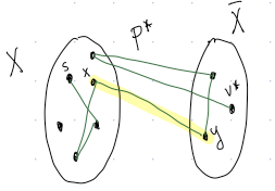
In Figure 4, the first edge in \(C\) to appear in \(P^*\) is highlighted - the edge \((x,y)\). We can divide up this path into two segments, the part of the path from \(s\) to \(y\), and the part of the path from \(y\) to \(v^*\). Then the total length of this path \(L(P^*)\) is the sum of these two lengths: \[ L(P^*)=L(s\rightarrow y)+L(y\rightarrow v^*). \] We have that \[ L(s\rightarrow y)\geq ....???\\ L(y\rightarrow v^*)\geq ...??? \]
Thus \(L(P^*)\geq L(P)\), contradicting the fact that \(P\) is not optimal. Thus in fact, \(P\) must have been optimal, and the assignments of the algorithm for up to \(k+1\) elements in \(X\) must be optimal.
5 Runtime of Dijkstra’s Algorithm
5.1 Group work
- What data structures should you use to improve the algorithm and why?
5.2 MinHeap Set-up
We will use a MinHeap and store Vertex objects in the heap.
We will create a Vertex object with the following attributes:
* name
* key
* prior
We will create such an object for each \(v\in \bar{X}\). For a vertex \(v\), the attributes should be set to:
* name: \(v\)
* key: \(\textrm{min}_{u\in X}L[u]+w(u,v)\)
* prior: \(\textrm{argmin}_{u\in X}L[u]+w(u,v)\)
Consider the following snapshot of variables in the algorithm:
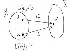
In this situation, what should \(v.prior\) be set to?
A) \(u\)
B) \(w\)
C) \(15\)
D) \(8\)
We will put Vertex objects into the MinHeap according to their key values.
Recall the properties of a Min Heap:
- You can initialize \(n\) items in the heap in \(O(n\log n)\) time
- You can remove ~the item with the minimum key value~ any item in \(O(\log n)\) time, as long as have pointer to that element of the heap.
- You can insert a new item into the heap in \(O(\log n)\) time.
5.3 Modifying the Pseudocode to Incorporate the MinHeap
HUFFMAN
Input: \(G=(V,E)\), \(s\in V\), \(w:E\rightarrow \mathbb{R}^+\), such that \(|V|=n\).
Output: n dimensional arrays \(L\) and \(P\) such that \(L[v]=\)length of shortest path from \(s\) to \(v\) in \(G\), and \(P[v]=\)shortest path from \(s\) to \(v\) in \(G\).// Initialization:
\(X\leftarrow\{s\}\) \(\quad\) // \(X\) is the set of visited/processed vertices
\(L[s]\leftarrow0\)
\(P[s]\leftarrow\emptyset\)// Initializing Heap
Create empty Heap \(H\)
For \(u\in V-\{s\}\):
\(\quad\) * If \((s,u)\in E\):
\(\qquad\) - \(u.key\leftarrow w(s,u)\)
\(\qquad\) - \(u.prior\leftarrow s\)
\(\quad\) * Else:
\(\qquad\) - \(u.key\leftarrow \infty\)
\(\qquad\) - \(u.prior\leftarrow \emptyset\)
\(\quad\) * Push \(u\) into \(H\)// Greedily Processing Vertices
While \(H\neq \emptyset\):
\(\quad\) // Process current vertex
\(\quad\) * \(u\leftarrow H.pop\)
\(\quad\) * \(X\leftarrow X\cup \{u\}\)
\(\quad\) * \(L[u]\leftarrow u.key\)
\(\quad\) * \(P[u]\leftarrow P[u.prior]+(u,prior,u)\) // Remove! See pset\(\quad\) // Update Heap
\(\quad\) * For \(v:(u,v)\in E\):
\(\qquad\) - Remove \(v\) from \(H\)
\(\qquad\) - If \(v.key>L[u]+w(u,v)\):
\(\qquad\)\(\qquad\) ~ \(v.key\leftarrow L[u]+w(u,v)\)
\(\qquad\)\(\qquad\) ~ \(v.prior\leftarrow u\)
\(\qquad\) - Reinsert \(v\) into \(H\)
Why do we need the section “Update Heap?” Each vertex \(v\) in \(\bar{X}\) is stored in the Heap, and its \(key\) should hold the vertex in \(X\) that results in the minimal Dijkstra criterion to the current vertex. However, after we have added a new vertex \(u\) to \(X\), it could be that now the vertex \((u,v)\) has the minimal Dijkstra criterion. We previously hadn’t considered this edge because until this round, \(u\) was not an element of \(X\). But because \(u\) is the only new vertex being added to \(X\), only edges originating at \(u\) might result in edges with better Dijkstra criterion, so we just need to go through and check the neighbors of \(u\) to see if any of them do better than what we currently have for Dijkstra criterion.
Why is the runtime of this pseudocode \(O((n+m)\log n)\) when the graph \(G\) is given as an adjacency list?
Note that this is an improvement over the Bellman-Ford runtime, which is \(O((n+m)n)\) with an adjacency list.