Path Integral Formalism

1 Learning Goals

Describe how quantum algorithms gain an advantage over probabilistic algorithms
Analyze circuits using the path integral formalism

2 Superposition

Is superposition the quantum secret sauce?

Superposition does seem pretty awesome. For example, suppose you have \(3\) qubits in the \(\ket{0}\) state, and you apply \(H\) to each. You will end up with the state \[ (H\otimes H\otimes H)\ket{000}=\ket{+}\ket{+}\ket{+}=\frac{1}{2\sqrt{2}}\left(\ket{000}+\ket{001}+\ket{010}+\ket{011}+\ket{100}+\ket{101}+\ket{110}+\ket{111}\right) \] So with three qubits, we can access 8 standard basis states - it seems like we have exponential scaling! For example, if we then apply a 3-bit function \(U_f\) to the state \(\ket{+}\ket{+}\ket{+}\ket{0}\), in one query, we can get information about all 8 function values.

But actually, this exponential scaling is not that special. Consider flipping a coin 3 times: there are 8 possible sequences of outcomes. Seems like we have exponential scaling!

Since both quantum and probabilistic systems seem to have this same ability to quickly access an exponentially large space, by comparing quantum and probabilistic systems, we can learn what it is about quantum systems that really gives them their speed up

	Quantum computing	Probabilistic Computing
state:	\(\sum_{i\in\{0,1\}^n}a_i\ket{i}\) such that \(\sum_{i\in\{0,1\}^n}\|a_i\|^2=1\), \(a_i\in\mathbb{C}\)	\(\sum_{i\in\{0,1\}^n}a_i\ket{i}\) such that \(\sum_{i\in\{0,1\}^n}a_i=1\), \(\quad a_i\geq 1\) (\(a_i\)’s are probabilities)
measurement:	Probability of outcome \(i\) is \(\|a_i\|^2\)	Probability of outcome \(i\) is \(a_i\)
gate:	unitary (preserves normalization, reversibility)	left stochastic (preserves normalization, positivity)

We will look at what happens if we try to do Deutsch’s algorithm with probabilistic gates instead of quantum gates.

3 Probabilistic Vs Quantum Computing

Recall Deutsch’s Algorithm:

Figure 1: Circuit diagram of Detusch’s Algorithm

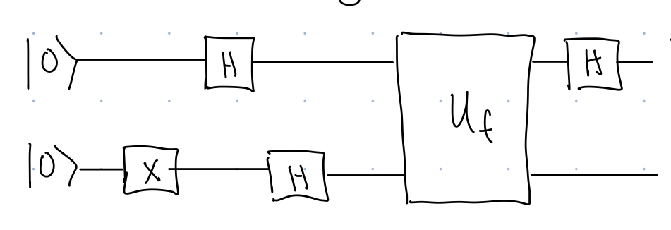
There are only 3 gates in Figure 1,

\(X\), \[\begin{align} \ket{0}&\rightarrow \ket{1}\\ \ket{1}&\rightarrow \ket{0} \end{align}\]
\(H\) \[\begin{align} \ket{0}&\rightarrow \frac{1}{\sqrt{2}}\ket{0}+\frac{1}{\sqrt{2}}\ket{1}\\ \ket{1}&\rightarrow \frac{1}{\sqrt{2}}\ket{0}-\frac{1}{\sqrt{2}}\ket{1} \end{align}\]
\(U_f\) \[\begin{align} \ket{0}\ket{0}&\rightarrow \ket{0}\ket{f(0)}\\ \ket{0}\ket{1}&\rightarrow \ket{0}\ket{\bar{f(0)}}\\ \ket{1}\ket{0}&\rightarrow \ket{1}\ket{f(1)}\\ \ket{1}\ket{1}&\rightarrow \ket{1}\ket{\bar{f(1)}}. \end{align}\]

Two of these gates, \(X\) and \(U_f\), are unitary and left stochastic, so are valid quantum or probabilistic gates. The only gate that is not probabilistic is \(H:\)

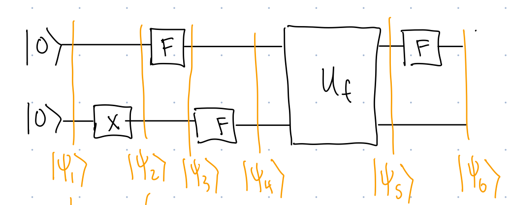
If we want to try to run Deutsch’s algorithm with a probabilistic computer, we will need to replace \(H\). We will replace it with the gate \(F\) (which takes any input and replaces it with an equal mixture of both \(\ket{0}\) and \(\ket{1}\)): \[ \begin{align} \ket{0}&\rightarrow \frac{1}{2}\ket{0}+\frac{1}{2}\ket{1}\\ \ket{1}&\rightarrow \frac{1}{2}\ket{0}+\frac{1}{2}\ket{1}. \end{align} \]

Now we have a circuit that we can run on a probabilistic computer:

3.1 Path integral analysis of probabilistic computation

To analyze this circuit, we will use a path integral approach. To do this we create a diagram of the four possible standard basis states:

After each gate, we use paths (lines) to show which other standard basis states the initial state is transformed into, and we put the the probabilities of each outcome state on the lines. Figure 2 shows how the diagram should look after applying the first three gates:

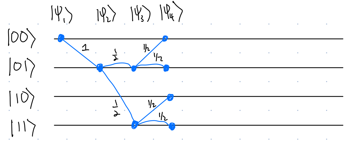
Figure 2: Path integral picture of the probabilistic circuit

To analyze the output of this probabilistic circuit:

Multiply probabilities on a path to get the probability of that path
Add probabilities of all paths terminating at a state to get the probability of that outcome

3.2 Path integral analysis of quantum computation

We can do the a similar path integral analysis of the quantum version of Deutsch’s algorithm. Figure 3 shows how the diagram looks after the first three gates

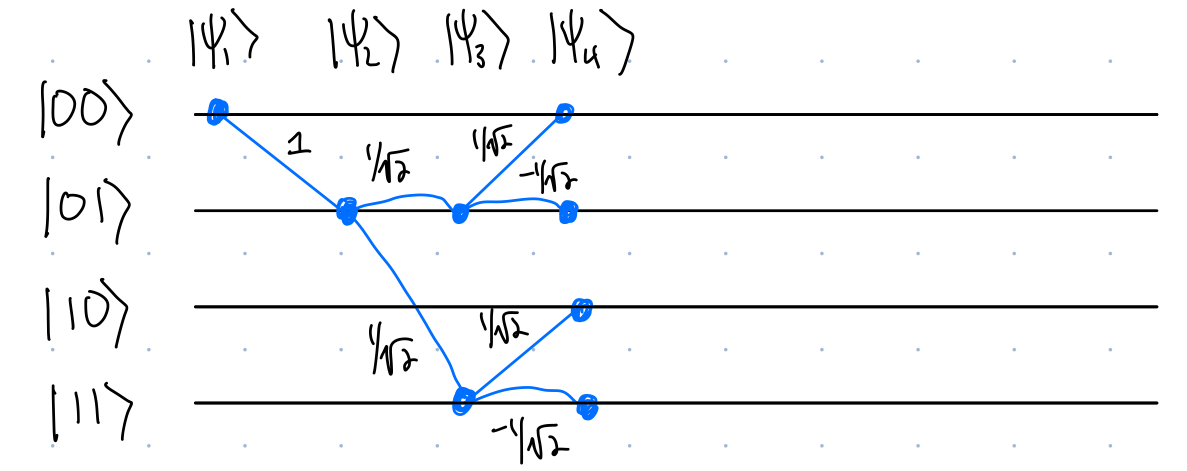
Figure 3: Path integral picture of the probabilistic circuit

To analyze the output of this quantum circuit:

Multiply ~~probabilities~~ amplitudes on a path to get the ~~probabilities~~ amplitude of that path
Add ~~probabilities~~ amplitudes of all paths terminating at a state, then take the absolute value squared, to get the probability of that outcome

Group Exercises

Finish filling out the two path diagrams (Figure 2 and Figure 3) in the case that \(f(0)=f(1)=1\), and in each case, calculate the probability of the 1st qubit being \(1\) at the end of the circuit.

Comparing these two diagrams, how would you describe the power of quantum computing versus probabilistic computing?