Grover’s Search Algorithm

Pre-class notes

In-class notes

1 Learning Goals

Practice analyzing the second most famous quantum algorithm using a geometric technique
Learn an important quantum algorithmic subroutine used in many quantum algorithms

2 Search Problem

Input: Query access to $f:\{0,1,2,\dots, N-1\}\rightarrow \{0,1\}$ such that

$\exists s:f(s)=1$
for all other $x\neq s$, $f(s)=0$

Output: $s$, the “marked item”

ABCD Questions

What is the classical query complexity (deterministic)?

$O(1)$
$O(\log{N})$
$O(N)$
$O(2^N)$

What is the classical query complexity (probabilistic)?

$O(1)$
$O(\log{N})$
$O(N)$
$O(2^N)$

3 Quantum Search Algorithm

The following figure shows the structure of the quantum algorithm for solving the Search Problem (Grover’s Algorithm).

Figure 1: Circuit Diagram of Grover’s Algorithm

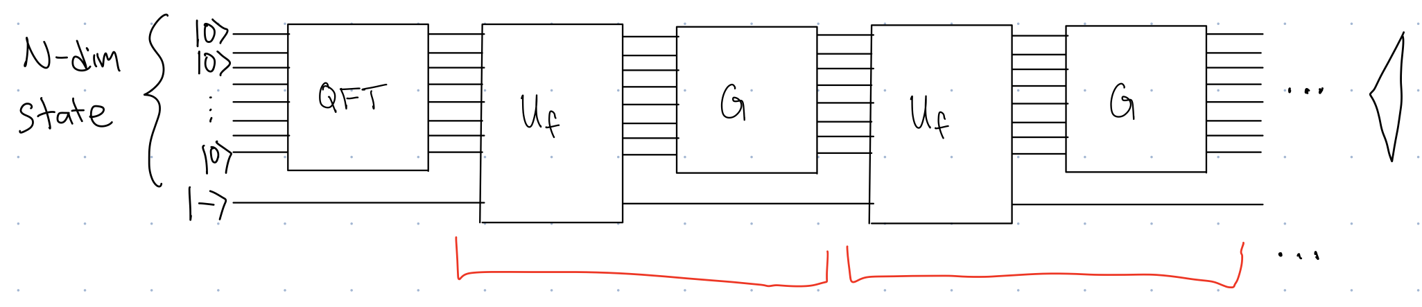
The pair of gates $U_f$ and $G$ are repeated some number of times (we will analyze to determine how many repeats are needed).

ABCD Question

How many qubits are needed for Grover’s algorithm to search for the marked item among the function’s $N$ inputs?

$\log_2N$
$\log_2N+1$
$N$
$N+1$

Because the final qubit entering $U_f$ is in the $\ket{-}$ state, we have the phase kickback effect that we saw in Deutsch’s algorithm: \[ U_f\ket{x}\ket{-}=(-1)^{f(x)}\ket{x}\ket{-}. \]

Because we only have one element $s$, such that $f(x)=1$, this can equivalently be written as \[ U_f\ket{x}\ket{-}= \begin{cases} -\ket{x}\ket{-}&\textrm{if } x=s\\ \ket{x}\ket{-}&\textrm{if } x\neq s. \end{cases} \]

In either case we see that the final qubit never changes from the $\ket{-}$ state, so we can think of $U_f$ as really only acting on the $N$-dimensional qubit state space. Thus, instead of $U_f$, we will consider an effective $U_f'$ that acts only on the first part of the system, and acts as: \[ U_f'\ket{x}= \begin{cases} -\ket{x}&\textrm{if } x=s\\ \ket{x}&\textrm{if } x\neq s. \end{cases} \]

We can write this $U_f'$ using ket-bra notation as: \[ U_f'=I-2\ketbra{s}{s}. \]

Let’s see why $U_f'=I-2\ketbra{s}{s}$ is the correct description of $U_f'$. We will look at how $U_f'$ acts on standard basis states. Consider $U_f'\ket{s}$: \[ \begin{align} U_f'\ket{s}=&(I-2\ketbra{s}{s})\ket{s}&\\ =&I\ket{s}-2\ketbra{s}{s}\ket{s}&\textrm{ Distribute}\\ =&\ket{s}-2\ket{s}(\braket{s}{s})& \textrm{ Associativity of bra/kets}\\ =&\ket{s}-2\ket{s}&\\ =&-\ket{s}. \end{align} \] so we see $U_f'$ acts as it should on $\ket{s}$. Likewise \[ \begin{align} U_f'\ket{x\neq s}=&(I-2\ketbra{s}{s})\ket{x\neq s}&\\ =&I\ket{x\neq s}-2\ketbra{s}{s}\ket{x\neq s}&\textrm{ Distribute}\\ =&\ket{x\neq s}-2\ket{s}(\braket{s}{x\neq s})& \textrm{ Associativity of bra/kets}\\ =&\ket{x\neq s}.&\textrm{ orthogonality of differing standard basis states}\\ \end{align} \]

We similarly define $G$, which is called the Grover Diffusion Operator, using ket-bra notation: \[ G=-I+2\ketbra{\alpha}{\alpha}\qquad \textrm{where }\ket{\alpha}=\frac{1}{\sqrt{N}}\sum_{i=0}^{N-1}\ket{i} \] where $\ket{\alpha}$ is the equal superposition state. We can likewise express $G$ as \[ G\ket{\gamma}= \begin{cases} \ket{\gamma}& \textrm{if } \ket{\gamma}=\ket{\alpha}\\ -\ket{\gamma}& \textrm{if } \braket{\gamma}{\alpha}=0 \end{cases} \]

3.1 Geometric Analysis of Grover’s Algorithm

While the state lives in a $2N$ dimensional space, in this particular algorithm, it only stays in $2$ of those dimensions. In particular, throughout the entire algorithm (after the first QFT), we can always express the state of the system at any point $i$ in time as: \[ \ket{\psi_i}=a_i\ket{\beta}+b_i\ket{s}, \quad a_i,b_i\in \mathbb{R} \] where \[ \ket{\beta}=\frac{1}{\sqrt{N-1}}\sum_{i\neq s}\ket{i}. \]

Helpfully, it is also easy to visualize objects that only live in 2D; we can draw them!

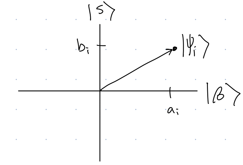
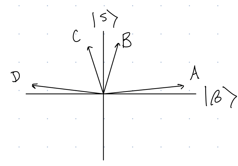
Figure 2: 2D representation of state of system during Grover’s algorithm. A vector represents the state, where a represents the x-component and b represents the y-component

ABCD Question

Where should $\ket{\alpha}=\frac{1}{\sqrt{N}}\sum_{i=0}^{N-1}\ket{i}$ be drawn on this diagram?

We can express the effects of $U_f'$ and $G$ as transformations of vectors in this space:

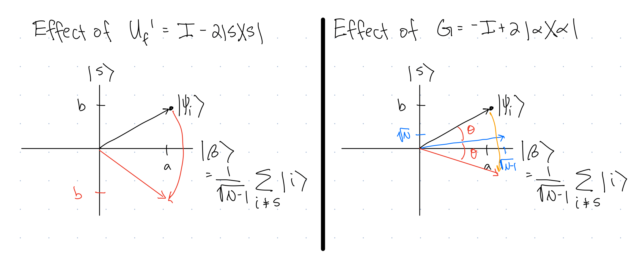
Note that these gates are both reflections in this space.

Group Exercise

How many iterations of $U_f'$ and $G$ should be applied before the state becomes very close to $\ket{s}$? Note:

Start with the state at $\ket{\alpha}$ (the state after the QFT is applied)
Consider the angle by which the state moves after the two reflections
You should assume $N$ is large.
It is helpful to know that $\tan^{-1}(x)\approx x$ for $x<<1$

3.2 Applications (Uses and Limits)

Important

Grover’s algorithm searches for the input to a function that gives a particular desired output. It is not a search through data. It is an open question whether quantum computers can speed up searches through data.

Despite Grover’s algorithm being limited to searching through function inputs and not through data, it is very useful at speeding up many types of algorithms.

For example, consider a classical algorithm that succeeds with probability $p$. A probabilistic algorithm can be though of as a function that takes in a random bit string representing a series of coin flips, and based on those coin flips makes a series of random choices within the algorithm. Then we can define \[ f(c)= \begin{cases} 1 &\textrm{ if coin flips sequence $c$ leads to a successful outcome}\\ 0 &\textrm{ else} \end{cases} \] If the algorithm succeed with probability $p$, that means that with fraction $p$ of possible bit strings $c$, $f(c)=1$. This algorithm can succeed in time $O(1/p)$ (by randomly choosing coin flip sequences until you find one that is successful, which happens after about $1/p$ repetitions).

Now we can create a quantum version of this algorithm that searches for a good coin-flip sequence. It can do this in $O(1/\sqrt{p})$ time.

For example, the best classical algorithm for 3-SAT (an NP-complete problem, is a probabilistic algorithm that succeeds with probability $p=(3/4)^n$), giving a runtime of $O((4/3)^n)$ (exponential). Using Grover’s algorithm, we can create a quantum algorithm that succeeds with probability $O((2/\sqrt{3})^n)$, which is still exponential, but much better scaling.

Because we can do this trick for so many algorithms, it is not particularly interesting from a theoretical perspective. It is also only a square root speed-up, which is not as exciting as an exponential speed-up. However, it would become interesting if quantum computers get fast enough that they could start solving some problems faster than classical algorithms using Grover’s algorithm. But we are very far from that point.