Deutsch’s Algorithm

\[ \newcommand{\braket}[2]{\langle{#1}|{#2}\rangle} \]

Pre-class notes

In-class notes

1 Learning Goals

• Design and analyze a quantum algorithm
• Read circuit diagrams
• Describe time and query complexity

2 Deutsch’s Problem and Query Complexity

The problem input is a \(1\)-bit function \(f:\)

\(x\)	\(f(x)\)
\(0\)	\(f(0)\)
\(1\)	\(f(1)\)

where \(f(0),f(1)\in\{0,1\}\)

For example, if we interpret \(x=0\) to be the daytime, and \(x=1\) to be the nighttime, an example of a \(1\)-bit function is:

\[ f(x)= \begin{cases} 1 &\textrm{if it will rain at time $x$}\\ 0&\textrm{if it will not rain at time $x$} \end{cases} \]

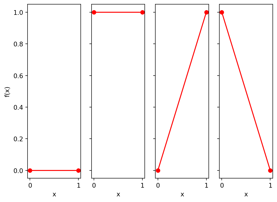
There are only 4 possible 1 bit-functions:

We call the first two functions “flat” (in the literature they are called “even”), and we call the second two functions “sloped” (in the literature they are called “balanced”).

Definition 1 Deutch’s Problem: Given query access to a \(1\)-bit function \(f\), determine if \(f\) is flat or sloped.

2.1 Classical Algorithm and Query Complexity

The following is a classical circuit diagram for Deutsch’s problem. Time goes from left to right, arrows represent bits of data, and boxes represent operations on bits. The circuit outputs \(1\) if \(f\) is flat, and \(0\) if \(f\) is sloped.

flowchart LR
START[0] --> B((f))
START --> C>NOT]
C --> D((f))
B --> E[AND]
B --> F>NOT]
D --> E[AND]
D --> G>NOT]
G --> H[AND]
F --> H[AND]
E --> I{OR}
H --> I{OR}
I --> J:::hidden

classDef hidden display: none;
style START fill-opacity:0, stroke-opacity:0;

Notice that this circuit uses the function \(f\) twice. We call each of these uses of \(f\) a “query”, because we are asking questions about the output of \(f\). Because the circuit calls the function \(f\) twice, we say

The query complexity of the circuit is: \(2\)

The time complexity of the circuit is: ??

The time complexity is how long it takes the circuit to run. This is extremely device dependent, as it depends on whether parallel computation is allowed, and it is dependent on the time needed to implement \(f\).

For this problem, we will want to minimize the query complexity. This is a reasonable thing to do if evaluating the function \(f\) is likely to take much longer than the other operations in the circuit.

ABCD Question

What is the minimum number of classical queries to \(f\) needed to determine if \(f\) is flat or sloped?

1. 0
2. 1
3. 2

We will find that for Deutsch’s problem:

• Classical Query Complexity: 2
• Quantum Query Complexity: 1

Why do we care about an improvement from \(2\) to \(1\)??

• Shows an advantage for quantum computing in a scenario where is seems impossible to get away with fewer than \(2\) queries.
• The algorithm for solving this problem uses techniques that are used in more complex algorithms. If you can understand this algorithm, it will help you to understand other algorithms, and build you intuition for how quantum algorithms work.
• If \(f\) is really really hard to compute, this could be practically of use. (\(1\) year is a lot less than \(2\) years, in terms of computational time.)

3 Quantum Gates (Circuit Picture)

3.1 Basic Circuit Elements

In quantum circuit diagrams:

• time goes from left to right
• each “wire” represents a qubit
• gates and measurements are boxes/shapes that intersect the qubit lines

Initialization of a qubit is represented as:

\(\ket{0}\bullet\hspace{-.22cm}-\hspace{-.22cm}-\hspace{-.22cm}-\)

where we almost always initialize qubits in the state \(\ket{0}\).

The single qubit gates (\(I\), \(X\), \(Y\), \(Z\), and \(H\)) we learned about in Quantum Gates are represented as

flowchart LR
START2[s]:::hidden --- B2[I]
B2 --- END2[t]:::hidden

START[s]:::hidden --- B[X]
B --- END[t]:::hidden

START1[s]:::hidden --- B1[Y]
B1 --- END1[t]:::hidden

START3[s]:::hidden --- B3[Z]
B3 --- END3[t]:::hidden

START4[s]:::hidden --- B4[H]
B4 --- END4[t]:::hidden

classDef hidden display: none;

The CNOT gate is represented as

Diagram of CNOT gate. The solid circle is the control qubit, and the open circle is the qubit that is acted on

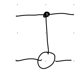
and measurements (which are always in the standard basis: \(M=\{\ket{0},\ket{1}\}\)) are represented as

Diagram of standard basis measurement

3.2 Quantum \(f\) Gate

It seems like a natural gate to use for querying the \(1\)-bit function \(f\) is the single qubit gate:

\[ \begin{align} \ket{0}&\rightarrow\ket{f(0)}\\ \ket{1}&\rightarrow\ket{f(1)}\\ \end{align} \tag{1}\]

Group Exercise

Explain why Equation 1 is not an allowed quantum gate. (Recall a gate should take quantum states to quantum states, and should be reversible.)

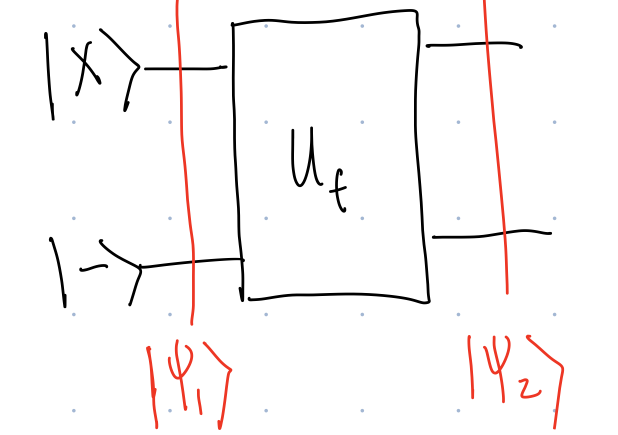
Instead, we will use the following gate:

Figure 1: Circuit representation of the f gate.

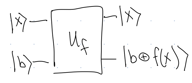
The way to interpret Figure 1 is that \(\ket{x}\) and \(\ket{b}\) must each be a standard basis state. In that case, \(U_f\) transforms them into \(\ket{x}\) and \(\ket{b\oplus f(x)}.\) We can also write the action of \(U_f\) as \[ \ket{x}\ket{b}\rightarrow\ket{x}\ket{b\oplus f(x)}. \tag{2}\] or \[ U_f\ket{x}\ket{b}=\ket{x}\ket{b\oplus f(x)}. \tag{3}\] This notation is simply an abbreviation of the following information: \[ \begin{align} \ket{0}\ket{0}&\rightarrow \ket{0}\ket{0\oplus f(0)}=\ket{0}\ket{f(0)}\\ \ket{0}\ket{1}&\rightarrow \ket{0}\ket{1\oplus f(0)}=\ket{0}\ket{\bar{f(0)}}\\ \ket{1}\ket{0}&\rightarrow \ket{1}\ket{0\oplus f(1)}=\ket{1}\ket{f(1)}\\ \ket{1}\ket{1}&\rightarrow \ket{1}\ket{1\oplus f(1)}=\ket{1}\ket{\bar{f(1)}} \end{align} \] Note that as usual, we only write how \(U_f\) acts on standard basis states. But this gives us enough information to determine how \(U_f\) acts on any state.

4 Developing an Algorithm for Deutsch’s Problem

Looking at Figure 1, we see that when the first/top qubit is \(\ket{0}\) we get information about \(f(0)\), and when the first/top qubit is \(\ket{1}\) we get information about \(f(1)\). Thus it seems like using superposition would be a good idea. With superposition, with a single query, we could get information about both \(f(0)\) and \(f(1).\) For example, let’s consider sending the \(\ket{+}\) state into the top of the \(U_f\) gate.

We will try analyzing the following circuit involving 2 qubits:

Figure 2: An attempt at a quantum algorithm for Deutsch’s algorithm.

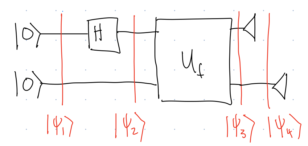
The way we analyze this circuit is to draw vertical lines through the circuit after each new gate is applied, and label these lines by states \(\ket{\psi_1}\), \(\ket{\psi_2}\), etc. Since time flows left to right, these lines represent the state of the system at a single point in time. We will start at the furthest line to the left and work our way to the right (i.e. work our way forward in time). Also, when we write \(\ket{0}\ket{0}\), the first (left) ket represents the top qubit and the second (right) ket represents the bottom qubit.

\[ \begin{align} \ket{\psi_1}&=\ket{0}\ket{0}\\ \ket{\psi_2}&=(H\otimes I)\ket{\psi_1}=(H\otimes I)\ket{0}\ket{0}=\ket{+}\ket{0}\\ \ket{\psi_3}&=U_f\ket{+}\ket{0}. \end{align} \]

We can see that the first part of the circuit sets up the superposition \(\ket{+}\) in the first qubit, and then we will apply the \(U_f\) gate, and then measure each qubit. We continue analyzing \(\ket{\psi_3}\). Perhaps the most common mistake I see in this class is:

\[ \begin{align} \textrm{DON'T DO THIS: }\quad \ket{\psi_3}&=U_f\ket{+}\ket{0}=\ket{+}\ket{0\oplus f(+)} \end{align} \] Looking at Equation 2, it seems like this is correctly following our description of how \(U_f\) should transform the state. However, Equation 2 is only a correct description of how the state transforms when the input states are standard basis states, and \(\ket{+}\) is not a standard basis state!! Instead, we must expand \(\ket{+}\) out in terms of standard basis states:

\[ \begin{align} \textrm{DO THIS: }\quad \ket{\psi_3}=U_f\ket{+}\ket{0}&=U_f\left(\frac{1}{\sqrt{2}}\ket{0}+\frac{1}{\sqrt{2}}\ket{1}\right)\ket{0}\\ &=\frac{1}{\sqrt{2}}U_f\ket{0}\ket{0}+\frac{1}{\sqrt{2}}U_f\ket{1}\ket{0}\\ &=\frac{1}{\sqrt{2}}\ket{0}\ket{f(0)}+\frac{1}{\sqrt{2}}\ket{1}\ket{f(1)}. \end{align} \]

Next, to get to \(\ket{\psi_4}\), we have a partial measurement, where we measure the top qubit. We get:

• Outcome \(\ket{0}\)
  • Probability: \(\left|\frac{1}{\sqrt{2}}\right|^2=1/2.\)
  • Sate collapses to \(\ket{0}\ket{f(0)}\). Since first qubit is destroyed, the second qubit is left in the state \(\ket{\psi_4}=\ket{f(0)}\).
• Outcome \(\ket{1}\)
  • Probability: \(\left|\frac{1}{\sqrt{2}}\right|^2=1/2.\)
  • Sate collapses to \(\ket{1}\ket{f(1)}\). Since first qubit is destroyed, the second qubit is left in the state \(\ket{\psi_4}=\ket{f(1)}\).

We see by the time we get to \(\ket{\psi_4}\) we not longer have information about both \(f(0)\) and \(f(1)\). Instead, we have information about one or the other. We have a 50/50 chance of either getting information about \(f(0)\) or about \(f(1)\). This situation is equivalent to flipping a coin, and then based on the outcome of the coin toss, deciding to either query \(f(0)\) or \(f(1)\).

Thus, superposition alone is not enough!

Group Exercise

Consider the following simple circuit.

The circuit is a graphical representation of \(\ket{\psi_2}=U_f\ket{x}\ket{-}\).

Show that when \(x\) is a standard basis state, \[ \ket{\psi_2}=(-1)^{f(x)}\ket{x}\ket{-}. \]

Next, use this fact to analyze the circuit in Figure 3, and show it solves Deutsch’s Problem:

Figure 3: Deutsch’s Algorithm

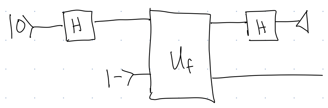
We see that Figure 3, the circuit that solves Deutsch’s Problem, only requires a single query to \(f\). We also see that it is not just superposition, but something about phases (complex amplitudes) is also important.

In the near future, we will study Deutsch’s algorithm from a different perspective in order to build intuition for why we get a quantum advantage.

4.1 Phase Kickback

Phase kickback is a key quantum subroutine. It is simply what we previously saw, that for a unitary \(U_f\), where \(f\) is a function with range \(\{0,1\}\), and for a standard basis state \(\ket{x}\), \[ U_f\ket{x}\ket{-}=(-1)^{f(x)}\ket{x}\ket{-}. \]

It is called phase kickback because we usually think of \(U_f\) as storing information about the value of the function \(f\) in the second qubit. However, here, information about the value of the function \(f\) is store in a phase (+1 or -1), that is kicked back to the front of the entire state, rather than the last qubit.