Lecture 1 - Introduction and Images
Logistics / Introductory Remarks
- About me
- About you - Informal poll questions:
- Do you all know each other?
- Have you taken machine learning (or similar)?
- Have you worked with numpy before?
- Have you worked with git before? Github classroom?
- Who got up before 7 this morning?
- Who's from the furthest away from Midd?
- Course webpage / syllabus: go/cs1053
- This points to https://www.cs.middlebury.edu/~swehrwein/cs1053_26w/.
- Also linked from the Syllabi tab on the Course Hub.
- Questions on the syllabus? About the course or anything else?
- Format remarks
- 3-hour classes(!)
- Aiming for 2 hours of instruction most days, with interactive / group work. I'll try to keep you awake!
- JupyterLab + whiteboard
- Lecture materials are in a public github repo: https://github.com/cs1053-26w/Lectures; also linked from Course Hub and course webpage.
- 3-hour classes(!)
Goals
- Know about a sampling of computer vision applications and understand the notion of vision tasks ranging from "low level" to "high level"
- Appreciate why computer vision is hard
- Know how images are formed under a simple pinhole camera model
- Understand how images are represented:
- On a computer
- In math
- Know how to represent color using different color spaces including RGB, HSV, and Lab
- Be able to write down mathematical image transformations that perform simple photometric or geometric manipulations of images functions
Lesson Plan
Quick introductions and day-1 logistics.
Logistics / introductory remarks
What is computer vision?
Why is it hard?
How are images formed?
break
Numpy crash course
How are images represented?
What can we do to images?
- Photometric transformations
- Geometric transformations
# Some basic setup
%load_ext autoreload
%autoreload 2

import os
import sys

# this makes it so we can import code files from the /src directory of this repo
src_path = os.path.abspath("../src")
if (src_path not in sys.path):
    sys.path.insert(0, src_path)
The autoreload extension is already loaded. To reload it, use:
  %reload_ext autoreload
# Library imports
import numpy as np
import imageio.v3 as imageio
import matplotlib.pyplot as plt
import skimage as skim
What comes to mind when you hear computer vision?
Brainstorm:
- images, visualization, editing
- recognition
- colors and shadow
- light transport simulation
- self-driving cars?
- evil drones
- face ID, face recognition
- pattern matching
- captchas
- optical character recognition
- image generation
- optical flow
- segmentation
- semantic segmentation, instance segmentation
Why are these hard problems?
- We humans have excellent visual systems built-in, and it's easy to take a lot of our capabilities for granted.
funny = imageio.imread("../data/obamafunny.jpg")
plt.imshow(funny)
<matplotlib.image.AxesImage at 0x1094de390>

Question to ponder: are we still really, really far?
Partial answer: ChatGPT session, December 2025
Our starting point:
Zoom in on the top left corner:
plt.imshow(funny[:12, :12, :])
<matplotlib.image.AxesImage at 0x10ebc4b30>

funny[:12, :12, 0]
array([[174, 169, 169, 167, 164, 162, 163, 164, 163, 162, 162, 164],
       [173, 169, 169, 166, 163, 162, 160, 158, 153, 152, 150, 149],
       [175, 171, 170, 169, 167, 165, 162, 158, 155, 150, 145, 142],
       [176, 172, 171, 171, 170, 168, 166, 162, 157, 150, 141, 136],
       [174, 171, 170, 170, 169, 168, 167, 164, 159, 149, 138, 131],
       [174, 170, 171, 171, 170, 169, 169, 167, 161, 151, 138, 131],
       [174, 168, 169, 171, 170, 169, 168, 167, 161, 153, 140, 129],
       [173, 168, 169, 169, 169, 170, 167, 165, 163, 155, 140, 124],
       [174, 170, 170, 169, 170, 169, 167, 165, 163, 155, 139, 117],
       [176, 172, 171, 171, 170, 167, 167, 166, 164, 156, 138, 112],
       [177, 171, 171, 171, 170, 168, 168, 166, 165, 156, 135, 110],
       [177, 171, 173, 172, 171, 171, 168, 166, 163, 155, 136, 110]],
      dtype=uint8)
Reasons vision is hard:
- Definitions - what is a cat even? (google image search for cat)
- Ambiguities - 3D to 2D projection, color vs lighting vs depth discontinuity
plt.imshow(funny[300:400, 500:550])
<matplotlib.image.AxesImage at 0x10ec1fc20>

- Scale
- images are big (MB)
- videos are bigger (GB)
- representative sets of images are even bigger than that (?? up to millions or billions of images)
# show size of funny
np.size(funny)
911250
HW problem 1:
Rank the following computer vision tasks from "low-level" to "high-level". There is not necessarily a single right answer, but there are many orderings we should all be able to agree on.
- Smoothing out graininess in an image without blurring the edges of objects
- For each pixel in a video frame, estimate the location of that pixel's content in the following frame (i.e., estimate per-pixel motion vectors, AKA optical flow)
- Labeling all the cats in a photo
- Generating an English language explanation of why an image is funny
- Brightening an image
- Reconstructing the 3D geometry of an object given photos from multiple perspectives
- Segmenting the foreground to create a background blur effect for videoconferencing
your thoughts here...
Break
GOTO L01A - numpy crash course
HW problem 2:
A (physical) pinhole camera is simply a box with a hole in it. Describe how the image would change if you made the distance from the pinhole to the back of the box longer or shorter. Assume the other box dimensions stay the same.
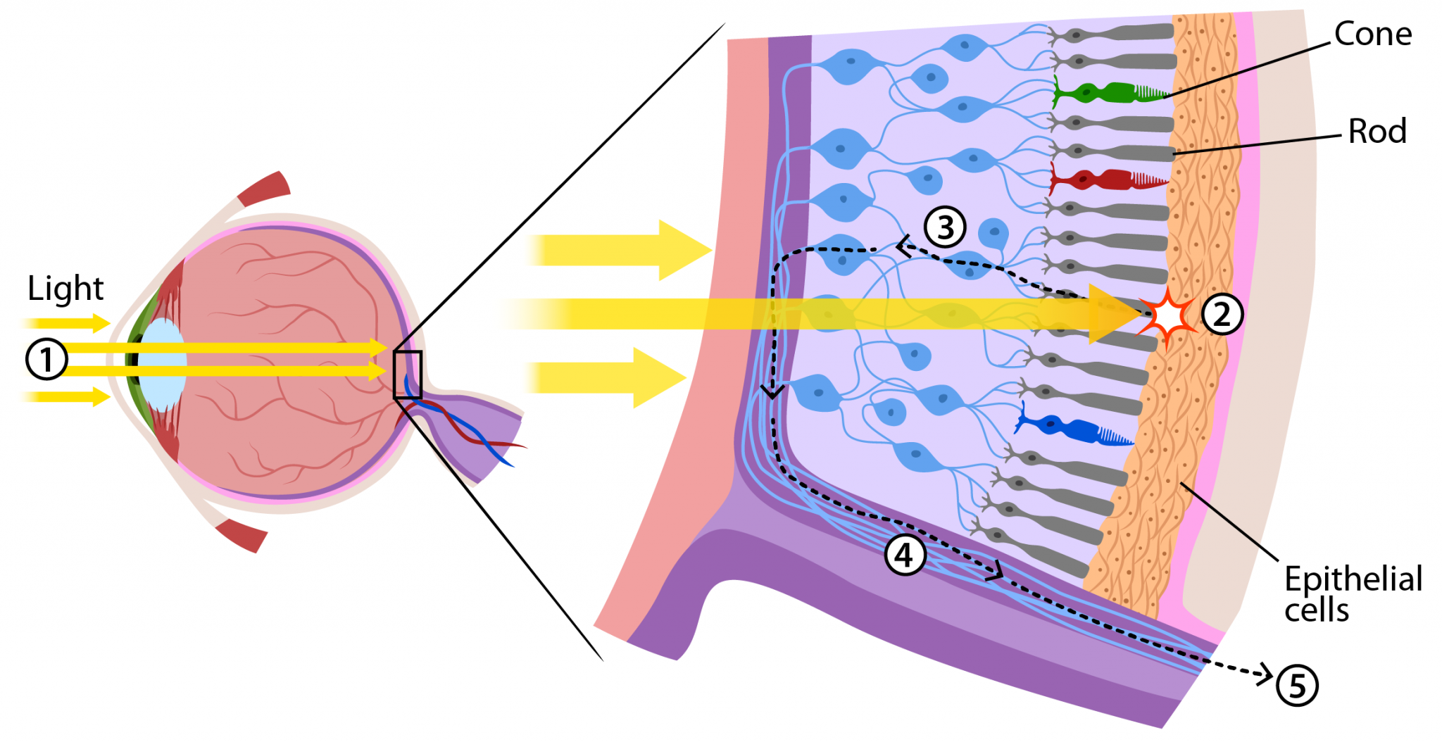
Image representation (whiteboard):
- Computationally:
ndarrayof size(height, width, 3) - Mathematically: a function mapping position to intensity (or color)
Grayscale image (one intensity value per pixel): $f: \mathbb{R}^2 \Rightarrow \mathbb{R}$
Color image (three intensity values per pixel): $f: \mathbb{R}^2 \Rightarrow \mathbb{R^3}$
A couple points of awkwardness when comparing this to an
ndarray:- What happens outside the image boundaries?
- What is the image's intensity value in between integer pixel indices?
- What range of intensity values are mapped onto distinguishable colors on a real display?
What is color?
Color theory is surprisingly deep. We'll just scratch the surface.
beans = imageio.imread("../data/beans.jpg")
plt.imshow(beans)
beans.shape
(600, 600, 3)

# look at a single pixel of beans
beans[0,0,:]
array([164, 150, 124], dtype=uint8)
# play with different rgb values
c = np.zeros((1,1,3))
c[:] = [0.5, 0, 0.8]
plt.imshow(c)
<matplotlib.image.AxesImage at 0x10ee2fe00>

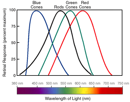
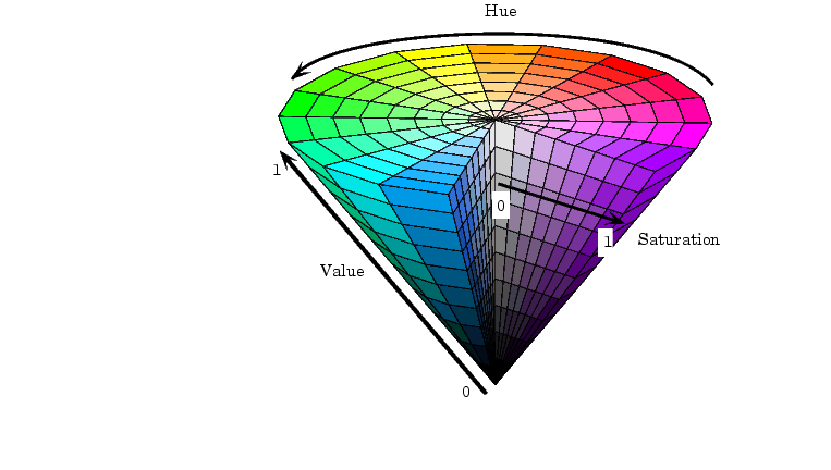
RGB: Not the only game in town
- You can think of RGB color as a cube: https://www.infinityinsight.com/product.php?id=91
- Pros: display (and vaguely human-eye) native, intuitive-ish
A couple other interesting color spaces:
Hue-Saturation-Lightness (HSL):
- Pros: intuitive control for color picking
CIE L*a*b*
- Pros:
- the L* channel is the luminance, or what the image should look like in "black and white"
- (mostly) perceptually uniform
- Cons: a* and b* give unintuitive control over color
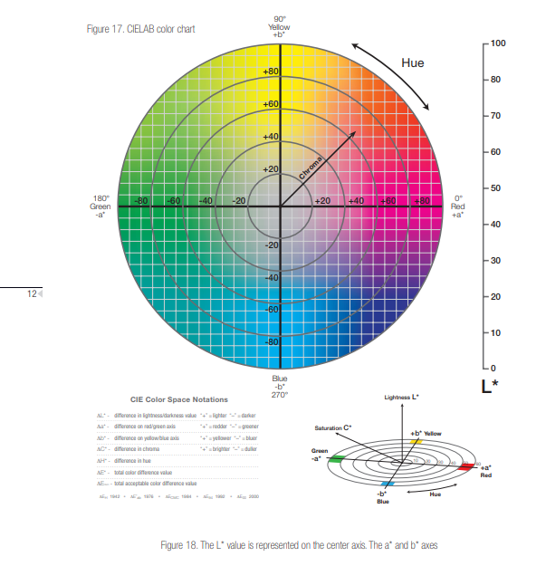
Interactive color picker with many color spaces: https://colorizer.org/
plt.imshow(skim.color.rgb2gray(beans), cmap="gray")
<matplotlib.image.AxesImage at 0x10ed21070>

# play with skim.color.rgb2hsv
plt.imshow(skim.color.rgb2hsv(beans)[:,:,0], cmap="gray")
<matplotlib.image.AxesImage at 0x10fd5bfe0>

# play with skim.color.
plt.imshow(skim.color.rgb2lab(beans)[:,:,0], cmap="gray")
<matplotlib.image.AxesImage at 0x10fe37e00>

beans.dtype
dtype('uint8')
beans.min(), beans.max()
(np.uint8(0), np.uint8(255))
An important note on datatype conventions
Most standard images (e.g., jpg, png, etc) are stored with 8-bit (1-byte) values for R, G, and B. If we want to do math (or anything!) to an image, we will get quantization error.
To avoid this, we always convert to floating-point values after loading.
The standard convention for the valid (displayable) range of floating-point values is 0 (darkest) to 1 (lightest).
For this reason, I wrote a little utility function:
# Codebase imports
# nb: the modification to sys.path at the top of the notebook makes these imports from ../src/ work
import util
import filtering
beans = util.byte2float(beans)
beans.dtype
dtype('float32')
beans.min(), beans.max()
(np.float32(0.0), np.float32(1.0))
# matplotlib obeys these dtype/range conventions:
# if it sees bytes, it assumes 0-255
# if it sees floats, its assumes 0-1 range
plt.imshow(beans)
<matplotlib.image.AxesImage at 0x11a1edc70>
What can we do to images?
One category: Photometric transformations - messing with the intensity values.
Suppose $g(x, y) = f(x, y) + .2$
or in other words,
g = beans + 0.2
How will $g$ compare to $f$?
g = beans + .4
plt.imshow(g.clip(0,1))
<matplotlib.image.AxesImage at 0x11a4ae900>

Brightness
$$ g(x, y) = s * f(x, y)$$
# implement filtering.brightness
g = filtering.brightness(beans, 2)
plt.imshow(g)
<matplotlib.image.AxesImage at 0x11a506810>

Thresholding
$$ h(x, y) = \begin{cases} 0 \textrm{ if } f(x, y) < t\\ 1 \textrm{ if } f(x, y) \ge t\\ \end{cases} $$
beans_gray = skim.color.rgb2gray(beans)

# implement filtering.threshold
g = filtering.threshold(beans_gray, 0.1)
plt.imshow(g, cmap="gray")
<matplotlib.image.AxesImage at 0x11a4ca120>

Homework Problems 5-6:
- Suppose you want to make an RGB color image stored in an array
amore saturated, without allowing any pixel values to go outside the range from 0 to 1. Write pseudocode (or python code) to implement this. - Given a grayscale image $f(x, y)$, how could you increase the contrast? In other words, how could you make the bright stuff brighter and dark stuff darker? Give your answer mathematically (not as code), and as above, your approach should not allow values to go outside their original range from 0 to 1; ideally you'll also avoid the need to clamp. Hint: try playing around with plotting some different functions on the input range $[0,1]$ to see if you can find one that does what we want.
Another category of image transformations: geometric transformations - messing with the domain of the function.
Example: $g(x, y) = f(-x, y)$
What would this look like?
And how would we write it in code?
plt.imshow(beans[:, ::-1, :]) # perform the above transformation
<matplotlib.image.AxesImage at 0x11a730a70>

Homework Problems 6-7:
- In terms of an input image $f(x, y)$, write a mathematical expression for a new image $g$ that is shifted four pixels to the left.
- In terms of an input image $f(x, y)$, write a mathematical expression for a new image $g$ that is twice as big (i.e., larger by a factor of two in both $x$ and $y$).