Polynomial-Time Reductions

1 Learning Goals

Reduce one problem to another
Define Polynomial Time Reduction
Describe why reductions are important

2 Cell Tower Transmission Problem

Input:

Array \(P\) such that \(P[i]\) is the location of the \(i^\textrm{th}\) cell tower.
Array \(D\) such that \(D[i]\) is the number of data packets tower \(i\) has in its queue.

Output: A set \(T\) of towers such that should broadcast in the next time step. Note that if two towers within 2 miles of each other broadcast at the same time, there will be interference of their signals.

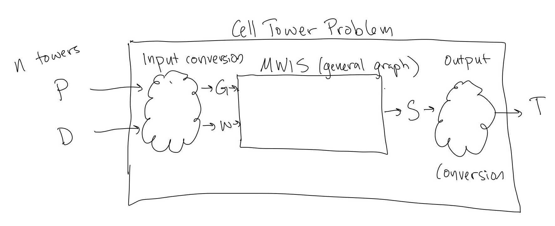
We would like to solve the Cell Tower Transmission Problem using a solver that solves MWIS. To do that, we need to turn the input to the Cell Tower Transmission problem into a MWIS input, and the we need to turn the resulting output from the MWIS solver back into a solution to our original problem. This process of converting one type of problem into another and back again is called a reduction (formal definition in next section). Graphically, this would look like:

Figure 1: Graphical representation of how the Cell Tower problem is converted to the MWIS problem

As a group, please discuss:

What should your input conversion and output conversion from Figure 1 be doing (generally), and why?
The social impact of implementing this Cell Tower transmission algorithm
- Stakeholders
- Who benefits
- Who is disadvantaged
- Cycles of reinforcement for winners/losers?
If you implement your conversion functions as algorithms, what are their asymptotic worst-case runtimes in terms of \(n\), the number of towers.

3 Polynomial-Time Reductions

We can more generally try to solve a problem \(P\) using a solver for problem \(Q\) by using an input conversion function \(f\) and an output conversion \(g\), as in Figure 2.

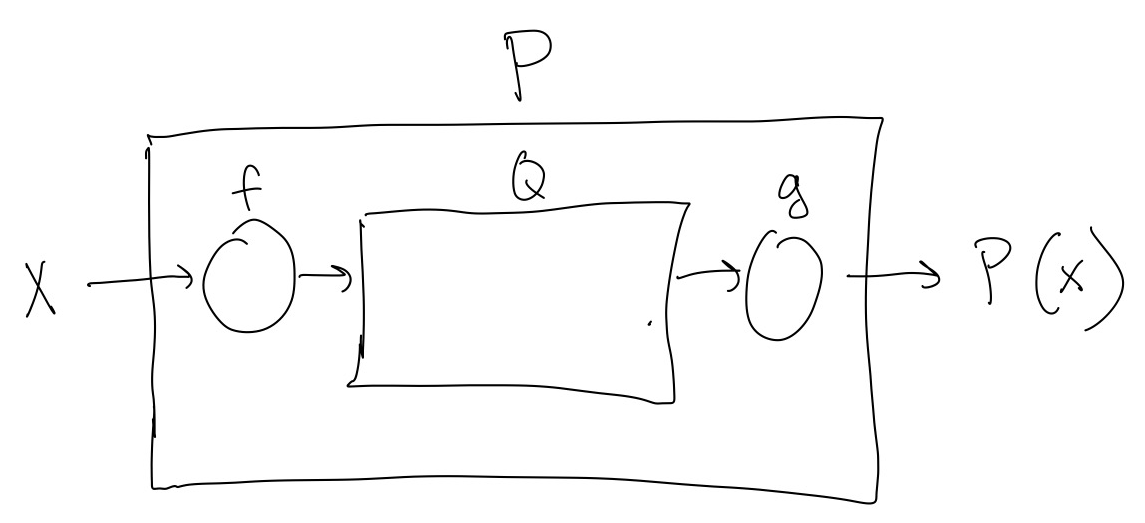
A smaller rectangular box labeled Q surrounded by a larger rectangular box labelled P. A small circle labeled f inside the P box to the left of the Q box, and a small circle labeled g inside the P box to the right of the Q box, with arrows pointing from left to right from outside the P box to the f circle, from the f-circle to the Q box, from the Q box to the g-circle, and then from the g circle to outside the P box. — Figure 2: Graphical depiction of a generic reduction from problem \(P\) to problem \(Q\)

However, this picture become a bit non-sensical if, for example, \(f=P\). In that case, the input conversion function is doing all of the work, and the solver for \(Q\) is not doing any work to solve the problem. This is not really the situation we want to consider. Thus, we consider reductions where the computational power of \(f\) and \(g\), the input and output conversion functions, are limited. This limitation ensures that the thing that is doing most of the work of solving \(P\) is the solver for \(Q\). Formally, we define a polynomial time reduction as:

Definition 1 If we can solve problem \(P\) with a solver for \(Q\) such that the runtime of the input and output conversion functions (\(f\) and \(g\) in Figure 2) have polynomial runtimes, we say “\(P\) is polynomial time reducible to \(Q\),” or “\(P\) reduces to \(Q\),” denoted by \(P\leq_p Q.\)

In the above definition, we use the term “polynomial runtime:”

Definition 2 We call \(O(n^d)\) for a constant \(d\) polynomial scaling.

Examples of polynomial runtimes in \(n\):

\(O(1)\)
\(O(n)\)
\(O(n\log n)\)
\(O(n^{10})\)

Essentially, we have limited the input and output conversion functions in our reduction to not be able to do things that take exponential time. From the perspective of exponential scaling, polynomial time scaling is practically nothing, trivial.

3.1 Remembering the direction of reduction

It can be hard to remember which problem is which when we say “\(P\) reduces to \(Q\),” or \(P\leq_p Q.\)

Let’s first try to keep track of what we mean when we write \(P\leq_p Q.\) To remember this, note that a solver for \(Q\) is so powerful, it can not only solve the problem \(Q\), it can also solve the problem \(P\) (with only a trivial) amount of extra work done by the input and output conversion functions. Thus a solver for \(Q\) is more powerful than a solver for \(Q\), and that is why \(Q\) is greater than \(P\).

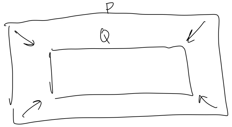
When we say “\(P\) reduces to \(Q\),” because the word “reduces” sounds like we are getting smaller, it can sound like the \(Q\) solver is less powerful, but this is the opposite of what we are trying to say. One way to remember is to draw a diagram like in Figure 3, and imagine the \(P\) box shrinking down (reducing) to the \(Q\) box. But at the same time, keep in mind that even though the \(Q\) box is smaller, it is the more powerful solver.

A smaller rectangular box labeled Q surrounded by a larger rectangular box labelled P with arrows pointing from the corners of P to the corners of Q. — Figure 3: Mnemonic picture for remembering direction of reduction from \(P\) to problem \(Q\)

3.2 Why do we care about reductions

There are two main reasons to care about reductions:

Practical: If we have a good algorithm for \(Q\) we can use it to solve \(P\) without having to code up an entirely new algorithm from scratch.
Conceptual: Reductions give us a way to compare the difficulty of problems and the resources needed to solve problems. If the resources needed to solve a problem \(Q\) can also allow us to solve a problem \(P\), then \(Q\) must be at least as hard to solve as \(P\), if not harder.