Huffman’s Encoding Algorithm

In-class notes

1 Learning Goals

• Describe “binary code,” “prefix free,” “average letter length”
• Explain connection between binary codes and binary trees
• Describe Huffman’s algorithm
• Analyze runtime of Huffman’s algorithm
• Describe impact of data structures on algorithm runtime
• Prove correctness of Huffman’s algorithm

2 Binary Codes and Binary Trees

Let \(\Sigma\) be a set containing the characters in an alphabet.

Definition 1 Given an alphabet \(\Sigma\), a binary code is a function \(f:\Sigma\rightarrow\{0,1\}^*\).

Some examples of binary codes are Morse Code, Braille, and ASCII.

Suppose you have a message where the letter “a” occurs 50% of the time, “b” occurs 30% of the time, and “c” occurs 20% of the time. Which is the best encoding for this alphabet?

1. \(f(a)=00\), \(f(b)=01\), \(f(c)=10\)
   
2. \(f(a)=0\), \(f(b)=1\), \(f(c)=01\)
   
3. \(f(a)=0\), \(f(b)=10\), \(f(c)=11\)

Definition 2 Given an alphabet \(\Sigma\), a probability function \(p:\Sigma\rightarrow\mathbb{R}\), and a binary encoding \(f\) of \(\Sigma\), the average letter length of \(f\) is \[ L(f)=\sum_{i\in \Sigma}|f(i)|f(i) \] where \(|f(i)|\) denotes the number of bits used by \(f\) to represent \(i\).

It turns out there is a one-to-one correspondence between binary codes and binary trees, as illustrated in Figure 1:

Figure 1: A binary code represented as a function and as a tree

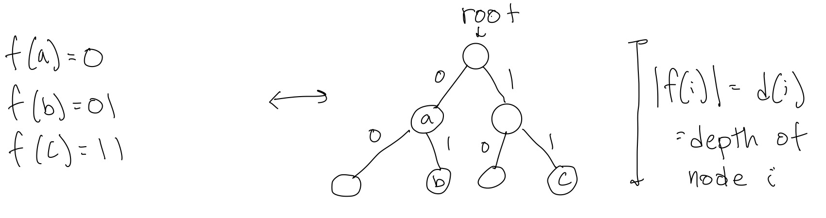
We see that trees can be helpful for decoding a binary code. To do this, you start at the root and based on the string of 0’s and 1’s that you read, you follow the corresponding edges until you get to a node with a letter in it, and you decode that sequence as a letter. However, this decoding doesn’t work well if there are two letters that both lie on the same path, as in Figure 1 where to get to node \(b\) you first have to pass through node \(a\). If you are decoding and see \(01\), you don’t know if that is an \(a\), followed by some other letter, or a \(b\).

This issue motivates the following definition, which ensures that we never have this ambiguity:

Definition 3 A code is prefix free if all letters are at leaves in the corresponding binary tree.

One easy way to create binary codes that are prefix free is to merge trees. To do this, start with each letter in the alphabet as a separate tree with just a single node, the root, labeled by that letter. Then at each round of the process, pick two of the trees and merge them into a single tree. Do this by creating a new root node and two edges coming out of the root, and attaching each tree to be merged to one edge of the new root. Continue until there is only one tree remaining, as in Figure 2:

Figure 2: Series of merges showing how to create a prefix free tree

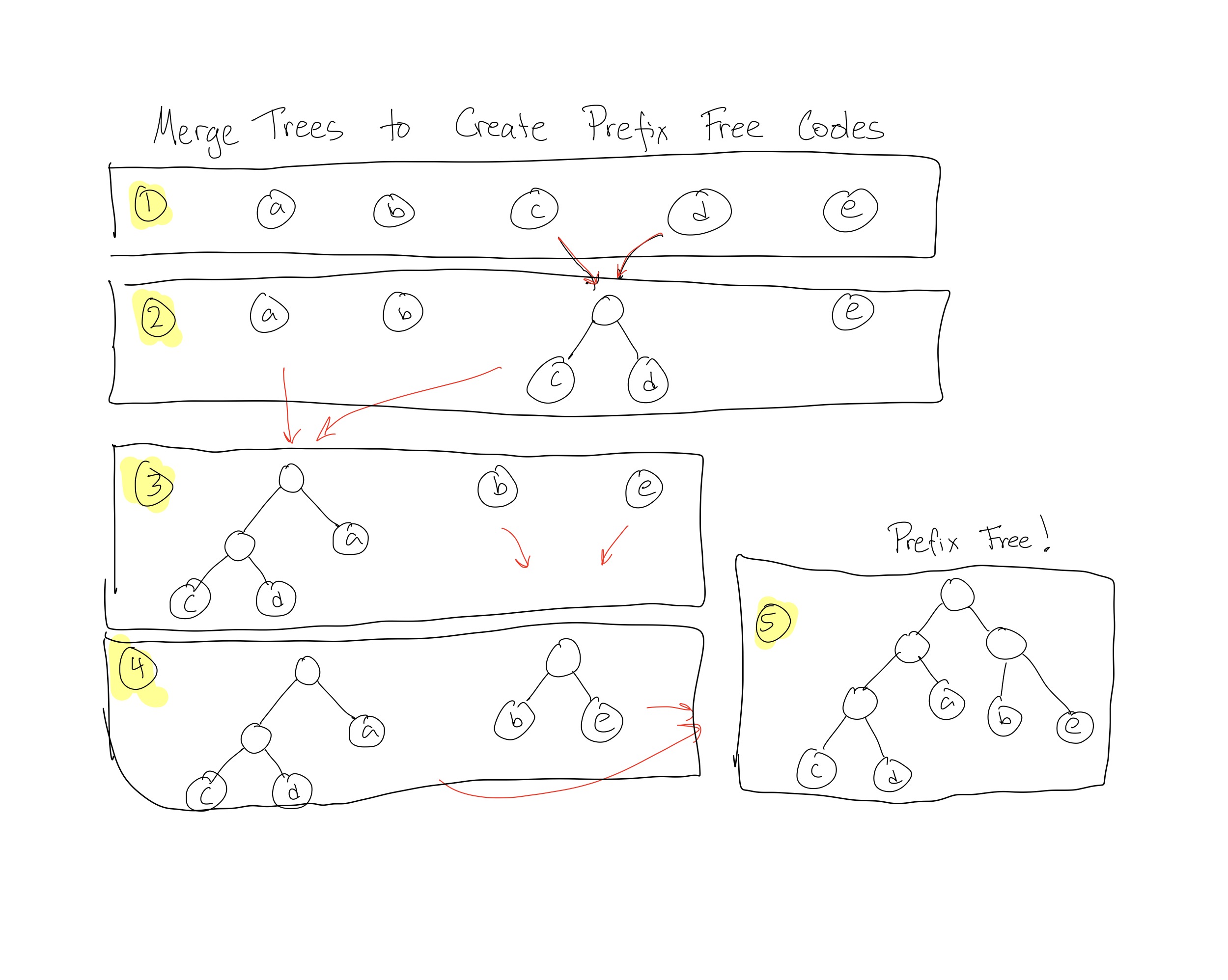
It turns out that any pre-fix free code can be created by such a series of merges.

3 Optimal Binary Encoding Problem and Huffman’s Algorithm

Now we can define our many problem, the Optimal Binary Encoding Problem

Input:

• An alphabet of symbols \(\Sigma\)
• \(p:\Sigma\rightarrow\mathbb{R}\), a probability for each symbol to appear

Output: A binary encoding \(f:\Sigma\rightarrow \{0,1\}\) such that

• \(f\) is prefix free
• \(f\) minimizes the average letter length among all prefix free binary codes

Now we can describe Huffman’s algorithm:

Huffman(\(\Sigma\), \(p\))
// Setting up our forest
For each \(i\in \Sigma\):
\(\quad\) * Create a tree with one node, labelled \(i\)
\(\quad\) * Give the tree weight \(p(i)\)
// Merging
While there is more than one tree in our forest:
\(\quad\) * Merge the two trees with the smallest weight
\(\quad\) * Set the weight of this new tree to be the sum of the weights of the two constituent trees

3.1 Practicing with Huffman’s Algorithms

• For the following alphabet, what binary code does Huffman’s create? What is the average letter length of this code?

\(i\)	\(p(i)\)
a	.3
b	.25
c	.2
d	.15
e	.1

• What is the runtime of Huffman’s algorithm in terms of \(|\Sigma|=n\)?
  
• Do you have any ideas for how to improve?
• Why is this a greedy algorithm?

3.2 Improved Runtime of Huffman’s Algorithm

As in the Closest Points problem, we can think about what aspect of the algorithm is causing a slowdown in the runtime, and think about whether there is a way we can reorganize the data to improve the runtime. In the Closest Points problem, we pre-sorted the data. Here, we can use a data structure to improve the runtime.

We first think about what aspect of the algorithm is causing the biggest slowdown in runtime. In our case, finding the trees with the smallest weight is what is driving the \(O(n^2)\) runtime.

But recall there is a data structure whose whole purpose is to make it easier to find the smallest element of a set of items: a Min Heap (also called a Priority Queue.)

A Min Heap has the following properties:

• You can initialize \(n\) items in the heap in \(O(n\log n)\) time
• You can remove the item with the minimum key value in \(O(\log n)\) time.
• You can insert a new item into the heap in \(O(\log n)\) time.

Now we can create a Min Heap where each object in the heap is a tree, and the key value of each object is the weight of the tree. Then the “Setting up the Forest” step takes \(O(n\log n)\) time, and each round of the “Merging” while loop takes \(O(\log n)\) time. There are still \(O(n)\) rounds of the while loop, giving us an \(O(n\log n)\) algorithm.

You now have everything you need to get started on Programming Assignment 2 (although you will need to figure out a lot of details.)

You will consider the social impact of Huffman’s algorithm in Programming Assignment 2.

3.3 Proof of correctness of Huffman’s Algorithm

To prove Huffmans algorithm, we will again use an exchange argument, but now our exchange argument will be embedded in an inductive proof! Exciting!

Theorem 1 Huffman’s Algorithm produces a prefix free code that minimizes the average letter length.

Proof. of Theorem 1.

We will prove correctness by induction on \(n\), where \(n=|\Sigma|\), the number of characters in our alphabet.

Base Case: If \(n=2\), there are only two characters, which we’ll label \(a\) and \(b\). Huffman will create a tree with one root node and two children, one for \(a\) and one for \(b\), corresponding to \(a\) and \(b\) getting assigned the binary strings \(0\) and \(1\). The average letter length is \(1\), which is the smallest possible, so this is optimal.

Inductive Step: Assume for induction that Huffman’s algorithm produces a prefix free code with minimal average letter length for any code with \(k\) characters. Consider an input with alphabet \(\Sigma\) such that \(|\Sigma|=k+1\).

Let \(a\), \(b\) be the elements of \(\Sigma\) with the smallest \(p\)-values (smallest probabilities/frequencies.) Define a new alphabet \(\Sigma^-\) where we remove the characters \(a\) and \(b\), and and add in a new character \(a/b\): \[\Sigma^-=(\Sigma\setminus\{a,b\})\cup\{a/b\}\] where the frequency of \(a/b\) is \(p(a/b)=p(a)+p(b).\)

Example 1  

• If \(\Sigma=\{e,f,g,h\}\), with \(p(e)=.1\), \(p(f)=.7\), \(p(g)=.15\), and \(p(h)=.05\),
  
• Then \(\Sigma^-=\{e/h, f, g\}\) with \(p(e/h)=.15\), \(p(f)=.7\), and \(p(g)=.15\).

Then we can consider how Huffman behaves in when creating a tree for \(\Sigma\) versus \(\Sigma^-\). For our example, we have:

Figure 3: Comparison of first few iterations of Huffman’s algorithm for \(\Sigma\) vs \(\Sigma^-\)

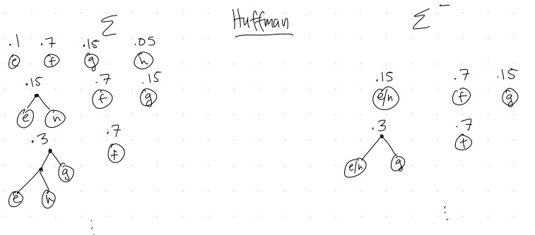
While Figure 3 is for a particular example, we can see that the general pattern will hold for every pair of \(\Sigma\) and \(\Sigma^-\): the trees produced will look almost exactly the same, except the subtree of \(a\) and \(b\) (the two smallest-weight trees), which will always get merged together in the first round of Huffman for \(\Sigma\) will be replaced by the single node \(a/b\) in the tree produced for \(\Sigma^-\).

Figure 4: The tree \(T\) produced by Huffman for \(\Sigma\) and the tree \(T^-\) produced by Huffman for \(\Sigma^-\). The are exactly the same except the subtree with \(a\) and \(b\) is replaced by a single \(a/b\) node.

Now by inductive assumption, \(T^-\) has minimal average letter length, because it is a Huffman tree with only \(k\) characters.

To continue the proof, we will need the following lemma:

Lemma 1 There is a minimal average letter length prefix tree where \(a\) and \(b\) are siblings (\(a\) and \(b\) are the characters with smallest \(p\)-value).

We will prove the Lemma 1 later.

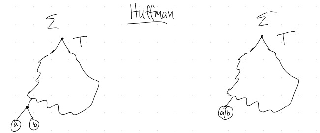
Now suppose for contradiction that \(T\) is not optimal. Then an optimal tree \(T^*\) exists such that \(T^*\neq T\). By Lemma 1, we can assume that \(a\) and \(b\) are siblings in \(T^*\). Then we will define a new tree \({T^*}^-\) that is exactly the same as \(T^*\) except with the subtree with \(a\) and \(b\) replaced by the single node \(a/b\), as in Figure 5.

Figure 5: The assumed optimal tree \(T^*\) for \(\Sigma\) and the tree \({T^*}^-\) that is the same as \(T^*\) except with the subtree with \(a\) and \(b\) replaced by the single node \(a/b\).

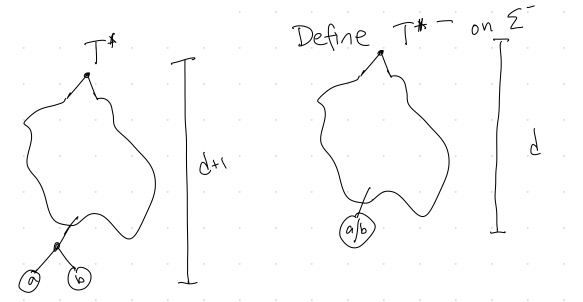
Then (fill in the ????’s in terms of \(d\), \(p(a)\), and \(p(b)\))

\[ \begin{align} L(T^*)&=\sum_{i\in\Sigma: i\neq a,b}p(i)d(i)+????\\ L({T^*}^-)&=\sum_{i\in\Sigma^-: i\neq a/b}p(i)d(i)+???? \end{align} \] So \[ L(T^*)-L({T^*}^-)= ???? \] Similarly \[ L(T)-L(T^-)= ???? \] Thus \[ L(T^*)-L({T^*}^-)=L(T)-L(T^-). \] Rearranging, we have \[ L(T)-L(T^*)=???? \] This is a contradiction because ????

Thus our assumption that \(T\) was not optimal must have been false, and in fact \(T\), the tree produced by Huffman’s algorithm for any alphabet with \(k+1\) elements must be optimal.

Therefore, by induction, we have that Huffman’s algorithm always produces a prefix free tree with minimal average letter length.

Now all that is left is to prove Lemma 1.

Proof. of Lemma 1.

Let \(T'\) be any optimal prefix free tree where \(a\) and \(b\) are not siblings. Let \(x\) and \(y\) be sibling leafs in \(T'\) at maximum depth, as in Figure 6.

Figure 6: Tree \(T'\).

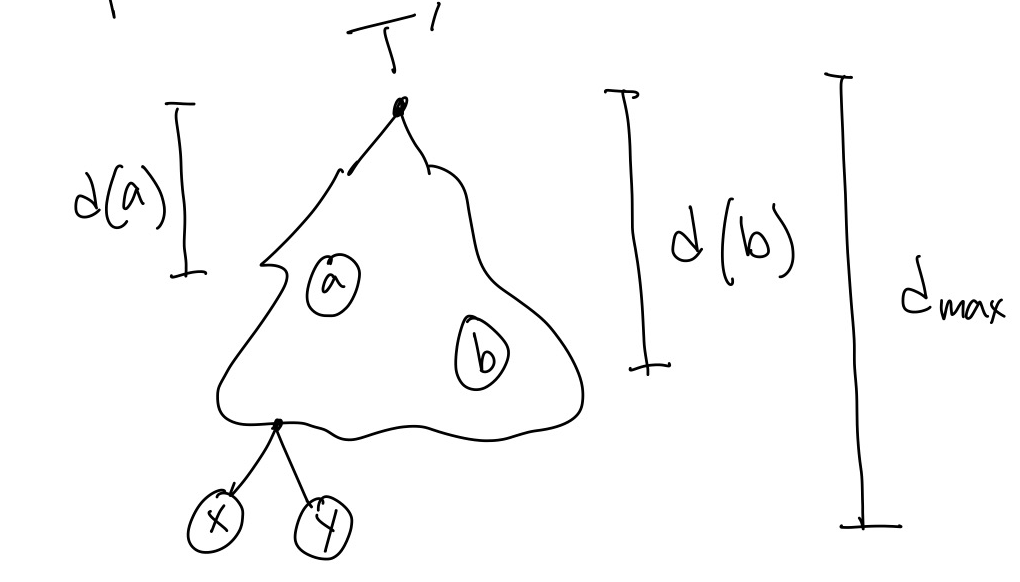
Create a tree \(T'_{ex}\) by exchanging \(x\) and \(a\), and exchanging \(y\) and \(b\), (\(ex\) for exchange). Then \(T'_{ex}\) will have the same or smaller average letter length as \(T'\) because…… (see pset)

Since \(T'\) was optimal, this means \(T'_{ex}\) must also be optimal, but it has \(a\) and \(b\) as siblings.