Shor’s Factoring (Period Finding) Algorithm
\[ \newcommand{\braket}[2]{\langle{#1}|{#2}\rangle} \]
1 Learning Goals
- Analyze a multi-qubit algorithm
- Become familiar with Shor’s factoring algorithm (the most famous quantum algorithm; its techniques are widely used in other algorithms)
2 Public Key Crypto - RSA
To motivate why we want to create a factoring algorithm, we need to return to our public key crypto system, where Alice wants to send a message \(m\in\{0,1\}^n\) to Bob and doesn’t want Eve to learn the message, even though Eve can learn everything that Alice sends to Bob.
Figure 1 shows the basic steps in implementing RSA crypto:
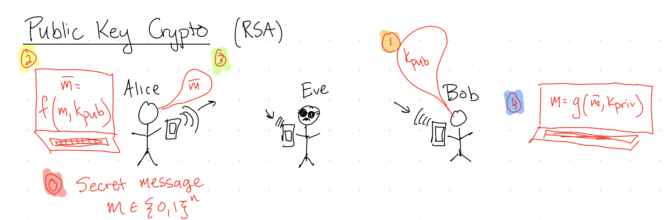
- Alice creates the message \(m\in\{0,1\}^n\) to send.
- Bob generates a public key and private key pair, and publicly broadcasts the public key \(k_{pub}\) for all to hear.
- Alice applies a function \(f\) to her secret message and Bob’s public key to get the encrypted message \(\bar{m}=f\left(m,k_{pub}\right)\).
- Alice sends \(\bar{m}\) across the public channel to Bob.
- Bob applies a function \(g\) to his private key and the encoded message to recover the original message: \(m=g\left(\bar{m},k_{priv}\right)\)
To determine the security of this crypto scheme, we need to think about what information Eve has access to. In this case, they have access to \(f_{pub}\) and \(\bar{m}=f\left(m,k_{pub}\right)\).
It turns out that if Eve could use \(f_{pub}\) and \(\bar{m}\) to determine \(m\), if only she could solve what seems like a simple problem: factoring.
For example, if I tell you to factor \(15\), the solution is \(3\) and \(5\). Seems easy, but now try to do it with the following number:
\[ 25195908475657893494027183240048398571429282126204032027777137836043662020707595556264018525880784406918290641249515082189298559149176184502808489120072844992687392807287776735971418347270261896375014971824691165077613379859095700097330459748808428401797429100642458691817195118746121515172654632282216869987549182422433637259085141865462043576798423387184774447920739934236584823824281198163815010674810451660377306056201619676256133844143603833904414952634432190114657544454178424020924616515723350778707749817125772467962926386356373289912154831438167899885040445364023527381951378636564391212010397122822120720357 \]
This is a 617 digit number. If you can factor it into its two factors, you win \(\$200,000\). No one has yet claimed the prize. (In fact, no one has yet claimed the prize for an easier 270 digit number. 250 digits is the largest prize claimed so far.) Multiplication is much easier than factoring, so once you come up with potential factors, you can easily check if you are correct.
In this unit, we will learn the quantum part of a quantum algorithm for efficient factoring
3 Period Finding
The actual quantum algorithm for factoring involves a quantum part and also classical pre- and post- processing that we will not get into. The quantum part of the algorithm is solving a slightly different problem, called “period finding.” Period finding is a subroutine used in algorithms for factoring. This is the part of the algorithm that quantum computers can solve much more quickly than classical computers.
Input: Query access to \(f:\{0,1,2,\dots, N-1\}\rightarrow \{0,1,2,\dots, W-1\}\) where
- \(f\) has unknown period \(r\)
- there are no repeated values within a period
- \(N>r^2\) (the period repeats many times within the function)
For example, \(f\) could look like:
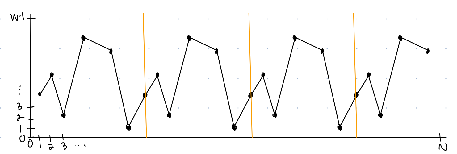
Output: \(r\), the period of \(f\)
What is the classical query complexity of factoring:
- \(O(\sqrt{r})\)
- \(O(r)\)
- \(O(r^2)\)
- \(O(N)\)
3.1 Bits to Digits
Classically, we code using digits (base 10), not binary, because binary is annoying to think in. We’ll do the same here: \[ \begin{align} 011&\leftrightarrow 3\\ \ket{011}&\leftrightarrow \ket{3}\\ \end{align} \]
Thus in this new notation, the standard basis states of the system are: \[\{\ket{0},\ket{1},\ket{2},\dots,\ket{N-1}\},\] and generic states are written as \[\ket{\psi}=\sum_{i=0}^{N-1}a_i\ket{i}, \quad \textrm{ s.t.} \sum_{i=0}^{N-1}|a_i|^2=1\]
Definition 1 When a system has \(N\) standard basis states, we say it is an \(N\)-dimensional system.
This does lead so some ambiguity. For example, if we have the state \(\ket{3}\), how do we convert this into binary?
- \(\ket{11}\)
- \(\ket{011}\)
- \(\ket{000000011}\)
To get around this ambiguity, we specify the dimension of our system
If \(\ket{3}\) is an \(N\)-dimensional state, how many qubits are in the system
- \(2\)
- \(O(\log N)\)
- \(O(N)\)
- \(O(2^N)\)
3.2 Quantum Circuit for Period Finding
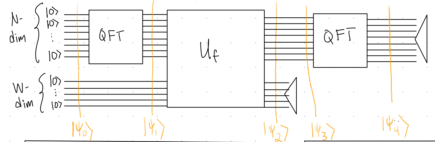
There are two new gates in this circuit, \(QFT\) and \(U_f\), where \(f\) is a function whose range is not \(\{0,1\}.\) Additionally, note that we think of the state of the algorithm as having two parts, an \(N\) dimensional part, and a \(W\) dimensional part.
We next describe the gates
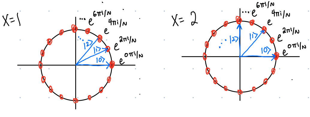
- \(QFT\). For \(\ket{x}\) an \(N\)-dimensional standard basis state: \[ \begin{align} QFT\ket{x}=\frac{1}{\sqrt{N}}\sum_{y=0}^{N-1}e^{2\pi i xy/N}\ket{y} \end{align} \]
In Figure 4, I show the amplitudes (before dividing by \(\sqrt{N}\)) of the output states when \(QFT\) is applied \(\ket{1}\) and \(ket{2}\). In both the left and the right figures, I have put in red the phases \(e^{0N\pi i/N}, e^{2\pi i/N},e^{4\pi i /N},e^{6\pi i /N},\dots\). In blue I have labeled the kets who have that amplitude. For example, when \(QFT\) is applied to \(\ket{1}\), we get \(\frac{1}{\sqrt{N}}\left(\ket{0}+e^{2\pi i/N}\ket{1}+e^{4\pi i /N}\ket{2}+e^{6\pi i /N}\ket{3},\dots\right)\) and when \(QFT\) is applied to \(\ket{2}\), we get \(\frac{1}{\sqrt{N}}\left(\ket{0}+e^{4\pi i/N}\ket{1}+e^{8\pi i /N}\ket{2},\dots\right)\).
[QC4 warm-up]
What state results when we apply \(QFT\) to the state \(\ket{0}\)?
The other new(ish) gate is \(U_f\). For \(f:\{0,1,2,\dots, N-1\}\rightarrow \{0,1,2,\dots, W-1\}\) and \(\ket{x}\ket{y}\) where \(\ket{x}\) is an \(N\)-dimensional standard basis state and \(\ket{y}\) is a \(W\)-dimensional standard basis state: \[ U_f\ket{x}\ket{y}=\ket{x}\ket{y+f(x)\mod W} \]
The other parts of the circuit are measurements in the standard basis. We will show how to make multiqubit standard basis measurements but in the case that we are using the digit representation instead of the bit representation:
- Measuring the entire state with a standard basis measurement:
- \(\sum_{x=0}^{N-1}a_i\ket{i} \longrightarrow\) Probability of outcome \(\ket{x^*}\) is \(|a_{x^*}|^2\)
- Partial measurement (\(B\) system):
- \(\sum_{x=0}^{N-1}\sum_{y=0}^{W-1}a_{xy}\ket{x}_A\ket{y}_B \longrightarrow\) Probability of outcome \(\ket{y^*}\) is \(P(\ket{y^*})=\sum_{x=0}^{N-1}|a_{xy}|^2\) (the sum of the absolute value squared of all amplitudes with the subscript \(y^*\))
- State collapse to \[ \frac{1}{\sqrt{P(\ket{y^*})}}\sum_{x=0}^{N-1}a_{xy^*}\ket{x}_A \] note the \(B\) system is destroyed by the measurement.
[QC5]
Analyze Figure 3 and determine the probability distribution of possible measurement outcomes.
3.3 From Circuit Output to Determining the Period:
Here is the full algorithm for period finding:
- Run the period finding circuit twice to get \(z_1=Nk_1/r\) and \(z_2=Nk_2/r\)
- Run GCD (greaest common divisor/Euclid’s Algorithm) on \(z_1\), \(z_2\) to get \(\tilde{r}\)
- Check that \(f(0)=f(\tilde{r})\)
- If yes, return \(\tilde{r}\)
- If no, return to step 1.
This algorithm will succeed with high probability (\(\approx 2/3\)) after a constant number of rounds.
3.4 Quantum and Classical Complexity
We analyze the query and time complexity of the period finding circuit:
Query Complexity: The query complexity depends on the period \(r\) (in the classical case:)
- Quantum: \(O(1)\)
- Classical: \(O(\sqrt{r})\)
Time Complexity: With some classical pre- and post- processing, we could use this circuit to factor a number between \(N/2+1\) and \(N\):
- Quantum: Each QFT takes time \(O\left(\log_2^2(N)\right)\), and instantiating \(U_f\) for the particular case of factoring takes time \(O\left(\log_2(N)\right)\), so the overall runtime is \(O\left(\log_2^2(N)\right)\).
- Classical: \(O\left(e^{O\left(\log_2^{1/3}N\right)}\right)\), using an algorithm called the number field sieve
3.5 Pesky Detail
We looked at the probability of getting an outcome \(z=kN/r\), but if \(N/r\) is not in \(\mathbb{N}\), then \(z\) is a fraction, and so it is not possible to get it as the outcome of a measurement. Since the outcomes of measurements are always \(\ket{x}\) where \(x\) is a natural number.
On your pset, you will look at what happens in this case.