Scheduling Problem

In-class notes

1 Learning Goals

• Describe typical properties of greedy algorithms
• Describe the scheduling problem, as well as related terms like “objective function,” “optimization problem,” and “completion time,” “scoring function,” “optimal order,” “greedy order”
• Create counterexample to a greedy ordering
• Describe the structure of an exchange argument and prove optimality of a greedy algorithm using an exchange argument
• Modify exchange argument in the case that scoring function is not unique.
• Analyze the runtime of a greedy scheduling algorithm

2 Introduction to Greedy Algorithms

There is not an agreed upon definition of greedy algorithms, and many algorithms that at first seem different from each other are all classified as greedy. Over the course of the semester we will see several examples, and this will hopefully give a better sense of what “greedy” means. However, I’ll give you an informal definition

Definition 1 (informal definition) A greedy algorithm sequentially constructs a solution through a series of myopic/short-sighted/local/not-global/not-thinking about-the-future decisions

Greedy algorithms often have the follow properties:

• Easy to create (non-optimal) greedy algorithms
• Runtime is relatively easy to analyze
• Hard to find an optimal/always correct greedy algorithm
• Hard to prove correctness

2.1 Order Problem

Greedy algorithms are frequently used to design algorithms for ordering problems, which are a subclass of optimization problems (ordering problems are a broad class of problems that are very general - we will look at a specific ordering problem shortly).

Definition 2 An optimization problem is a problem where you would like your solution to be better (according to some pre-decided metric) that any other possible/feasible solution.

Generic Ordering Problem

• Input: \(n\) items.
• Output: Ordering \(\sigma\) of the \(n\) items that minimizes (or maximizes) \(A(\sigma).\)

Definition 3 We call \(A(\sigma)\), the function that we want our output to maximize or minimize, the objective function

For example, the following figure shows the possible orders of 3 items, and made-up \(A\)-values for each ordering.

Figure 1: Example of A values for orderings of 3 items

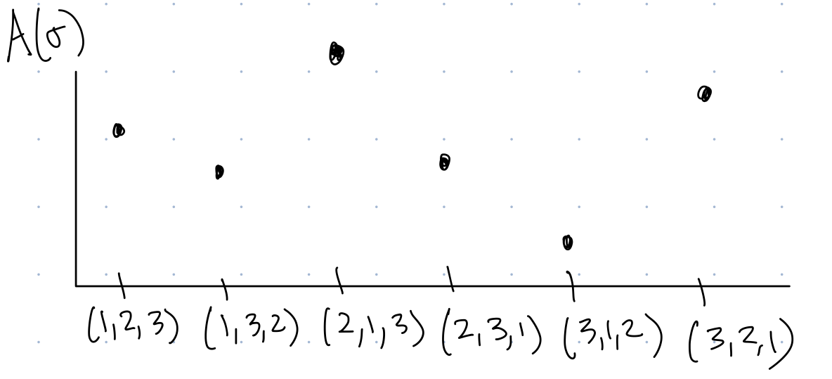
If our goal is to minimize \(A\), then for the example of Figure 1, the output of this ordering problem should be \((3,1,2)\), but if our goal was to maximize \(A\), then the output of this ordering problem should be \((2,1,3)\).

Here are two approaches for designing an algorithm to solve the Ordering Problem:

• Brute Force:
  • Evaluate \(A(\sigma)\) for every possible ordering of the \(n\) items. Keep track of the minimium (maximum) value found and the corresponding ordering, and then return that ordering.
  • Takes \(\Omega(n!)\) time (\(\Omega\) is asymptotic lower bound)
• Greedy
  • Design a simple scoring function \(f\). A scoring function is a function that maps each item to a score. Note that while the objective function maps orderings to numbers, the scoring function maps items to numbers.
  • Evaluate the score of each item
  • Return \(\sigma\) that puts the items in decreasing (increasing) order by score
  • Takes \(\Omega(n\log n)\) time.

3 Scheduling Problem

3.1 Description

The scheduling problem is a type of ordering problem.

For the scheduling problem, we imagine that we have a series of tasks that we want to accomplish, but we can only do one task at a time, and must complete that task before moving onto the next. Each task takes some amount of time (tasks can have the same or different times), and each task has a weight, which tells us the importance of that task. We would like to figure out how to schedule tasks to prioritize important, short tasks.

Input: \(n\) tasks. Information about the tasks is given in the form of two length-\(n\) arrays, one labeled \(t\), and one labeled \(w\). The \(i^\textrm{th}\) element of array \(t\) is the time required to complete the \(i^\textrm{th}\) task, which we call \(t_i\), and the \(i^\textrm{th}\) element of array \(w\) is the weight (importance) of the \(i^\textrm{th}\) task, which we call \(w_i\), where larger weight means more important. For example, we might have the input

task	1	2	3
time	3	4	2
weight	5	1	2

so in this case, \(t_1=3\) and \(w_3=2\)

Output: Ordering of tasks \(\sigma= (\sigma_1,\sigma_2,\dots,\sigma_n)\) that minimizes \[ A(\sigma)=\sum_{i=1}^nw_iC_i(\sigma), \tag{1}\] where \(C_i(\sigma)\) is the completion time of task \(i\) with ordering \(\sigma\), described below. Note that Equation 1 is the objective function for this scheduling problem

Assuming we start our first task at time \(0\), then run our sequence of tasks, \(C_i(\sigma)\) is the time at which the task \(i\) is completed when the tasks are done in the order given by \(\sigma\). For an example, suppose we have \[ t=(3,4,2) \] and consider the ordering \(\sigma=(3,1,2)\), so we do the third task first, then the first, and then the second. This is shown graphically in Figure 2:

Figure 2: Graphical representation of how jobs are ordered in time with ordering (3,2,1). Each job must be completed before the next can start.

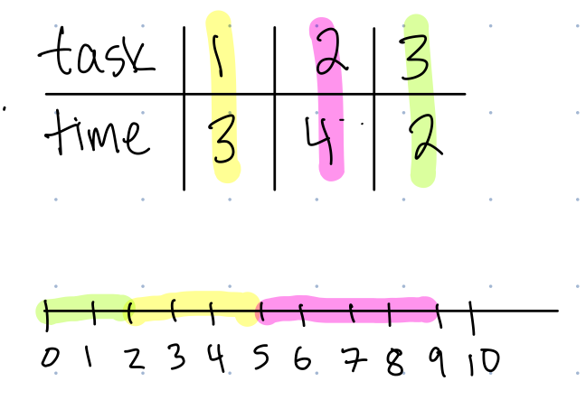
So \(C_3(3,1,2)=2\) because we do it first, it takes time \(2\), so it is completed at time \(2\). Next we do task \(1\), but it only gets started at time \(2\) after completing task \(3\), and runs until time \(5\), so \(C_1(3,1,2)=5.\) Now that task \(1\) is completed, we can finally do task \(2\) which takes another \(4\) time units, and so we complete it at time \(9\), so \(C_2(3,1,2)=9\). (When it is clear which ordering \(\sigma\) we are talking about, we will sometimes write \(C_i\) instead of \(C_i(\sigma)\).)

Application: Scheduling tasks on a single CPU (central processing unit) of a computer. Or scheduling your tasks…in the case that you must complete each task before moving on to the next.

ABCD Question

If \(t=(3,4,2)\) (the same example as above), what is \(C_3(2,1,3)\)

1. 2
2. 3
3. 7
4. 9

Group Exercises

1. Given the following input:

task	1	2
time	3	4
weight	5	1

What is the best order? (Use a brute force approach, and calculate \(A(\sigma)\) for all possible orderings.)

Hint: first calculate \(C_1\) and \(C_2\) for each ordering

2. What is the objective function \(A(\sigma)=\sum_{i=1}^nw_iC_i(\sigma),\) optimizing? (What time/weight jobs is it prioritizing?)

4 Creating Scoring Functions and Counterexamples

Creating a greedy algorithm is easy! All you need to do is come up with a scoring function that you think might optimize the objective function. This scoring function should be a function of the properties of each item. For our scheduling algorithm, this means the scoring function can depend on \(t_i\) and \(w_i.\)

For example, we can create the scoring function \[ f(i)=t_i \qquad \textrm{(increasing)} \tag{2}\] where we will order items from smallest time to largest time. This greedy algorithm will choose the ordering that puts the shortest jobs first, and the longest jobs last.

Done! We’ve designed a greedy algorithm!

Problem? It might not be a good algorithm. The greedy ordering, the ordering created by \(f\), might not be the optimal ordering, the one with the optimal \(A\) value.

In any case, it might not be good, but we can still practice creating a greedy algorithm using Equation 2. We first need to evaluate the score for each item (we’ll use our example input from the group exercise above):

task	1	2
time	3	4
weight	5	1
f	3	4

Since we have decided to order jobs in increasing \(f\)-value, our greedy ordering is \((1,2)\). In fact, when we did the brute force approach, we also found \((1,2)\) was the optimal ordering. This is great! Our greedy algorithm found the best possible ordering!!

Important

The scores, the \(f\)-values, of items mean nothing on their own. They can be negative, or 0, or positive, and it doesn’t tell you anything. Scores only have meaning when compared to the scores of other items.

4.1 Finding Counterexamples

Our greedy ordering was correct for the example above, but….will this greedy ordering always be correct?? To show that a scoring function will not always give us the optimal ordering, we can try to find a counterexample.

Tips for finding a counterexample:

• Think extreme
• Create tasks that are close in score but very different otherwise

Example

We will find a counter example to \(f(i)=t_i\) (ordered in increasing \(f\)-value).

We design the following set of jobs, that have very close times, but very different weights. In particular, we set the job that takes slightly longer to be much much more important.

task	1	2
time	1	2
weight	1	100
f	1	2

So in this case, our greedy ordering is again \((1,2)\).

However, if you do a brute force approach, you will find that actually, the optimal ordering for this input to the scheduling problem is \((2,1)\).

Group Exercises

Create counterexamples for the following scoring functions:

1. \(f(i)=w_i\) (decreasing)
2. \(f(i)=w_i-t_i\) (decreasing)

4.2 Design Approach

Here is a general approach for creating a good greedy algorithm:

1. Brainstorm several reasonable scoring functions. For example: \[ f(i)=w_i-t_i \textrm{ (decreasing)}\qquad f(i)=w_i/t_i \textrm{ (decreasing)}\qquad f(i)=w_i^2-2t_i \textrm{ (decreasing)} \] These are “reasonable” because they all tend to prioritize jobs that are important and short, which is our goal.
2. Test the scoring functions on examples, see how they do, and see if you can create counterexamples showing a scoring function is not optimal. (In some cases, you might also be satisfied with an algorithm that is not always optimal, but is close to optimal. For example, Prof. Das in her research often tries to show that an algorithm never does worse than 90% of the optimal value of the objective function.) These types of algorithms that are not always optimal or that you can’t prove are optimal, are called heuristics.
3. If you can’t find any counterexamples, you can try to prove that your greedy algorithm is correct.

5 Proving Correctness of Greedy Scheduling

Ordering jobs by decreasing value of \(f(i)=w_i/t_i\) is optimal for minimizing \(A(\sigma)=\sum_iw_iC_i(\sigma)\).

Proof. [We will use an “Exchange Argument,” which is a type of proof by contradiction]

Assume that \(w_i/t_i\) are distinct (i.e. no two jobs have the same score). Without loss of generality, we are going to relabel the tasks in decreasing score so that task \(1\) has the highest score, then task \(2\), etc, so that \[w_1/t_1>w_2/t_2>w_3/t_3\dots w_n/t_n.\] With this relabeling, we have that the greedy ordering is \[\sigma=(1,2,3,\dots,n).\] Assume for contradiction that \(\sigma\) is not the optimal ordering. Then there must exists another ordering \(\sigma^*\) that is the optimal ordering.

Since \(\sigma^*\neq \sigma\), there must be tasks \(b,y\in \{1,2,\dots,n\}\) where \(b<y\), but \(y\) appears immediately before \(b\) in \(\sigma^*\). In other words, \(b\) and \(y\) are in the wrong order, and right next to each other somewhere in \(\sigma^*\), so \(\sigma^*\) looks like: \[\sigma^*=(\dots, y, b, \dots).\] For example, if \(\sigma=(1,2,3)\), and \(\sigma^*=(3,1,2)\), then \(3\) and \(2\) are right next to each other but out of order, so we set \(y=3\) and \(b=1\).

Now let \(\sigma^{*'}\) be an ordering that is exactly the same as \(\sigma^*\) except that \(b\) and \(y\) are exchanges (i.e. swapped). Thus \(\sigma^{*'}\) looks like \[\sigma^{*'}=(\dots, b, y, \dots)\] where the \(\dots\) are the same sequence as in \(\sigma^*\).

Next we analyze \(A(\sigma^{*})-A(\sigma^{*'})\).

Group Exercise

Analyze \(A(\sigma^{*})-A(\sigma^{*'})\)

[See hand written notes for analysis.]

Thus we see that \(A(\sigma^{*})>A(\sigma^{*'})\). This is a contradiction because \(A(\sigma^{*})\) is optimal which meant it was supposed to have the smallest \(A\)-value of all orderings, but instead we see that \(A(\sigma^{*'})\) has a smaller \(A\)-value. Thus our original assumption, hat \(\sigma\) was not optimal, must have been incorrect, and in fact, \(\sigma\) must be the optimal ordering.

6 Big Picture: Exchange Argument Structure

Exchange arguments are commonly (although not always) used to prove the correctness of greedy algorithms. Here is the general structure of an exchange algorithm proof.

Exchange Argument

1. Let \(\sigma\) be the sequence that your greedy algorithm gives you, the one that you are trying to prove is optimal. For contradiction, assume it is not optimal.
2. Then that means there is some other sequence \(\sigma^*\) that is optimal.
3. But then at some point \(\sigma^*\) must be out of order relative to the greedy sequence. Create a new sequence \(\sigma^{*'}\) by exchanging two elements (or doing some other small change) of the sequence of \(\sigma^*\) to make it more like the greedy algorithm.
4. Show that \(\sigma^{*'}\) is better than \(\sigma^*\), a contradiction, since \(\sigma^*\) was supposed to be optimal. Thus our original assumption in step 1 that \(\sigma\) was not optimal must have been incorrect.

7 Continuing to Analyze our Greedy Scheduling Algorithm

7.1 Runtime of our greedy algorithm

ABCD Question

What is the runtime of our greedy scheduling algorithm?

1. \(O(1)\)
   
2. \(O(n)\)
   
3. \(O(n\log n)\)
   
4. \(O(n^2)\)

7.2 Loosening our Assumption

In our proof in Section 5, we assumed that no two tasks had the same value of \(w_i/t_i\).

Where did we use this assumption in our proof?

Without this assumption, we no longer have a contradiction!! (See hand-written notes for details.) But we can modify the proof so that it still works.

Proof. [Proof sketch] Choose some relabeling of the tasks so that \[w_1/t_1\geq w_2/t_2\geq w_3/t_3\geq\dots \geq w_n/t_n.\] We call \(\sigma=(1,2,3,\dots,n)\) our greedy ordering. Let \(\sigma^*\) be any other ordering. Then we will show that \(A(\sigma^*)\geq A(\sigma)\). Since we could choose any other ordering for \(\sigma^*\), this will show that \(\sigma\) has the same or better \(A\)-value compared to every other possible ordering, and thus \(\sigma\) is an optimal ordering.

Consider the following sequence:

By the logic of BubbleSort, if we continue to exchange out-of-order tasks, eventually we will eventually arrive at \(\sigma=(1,2,3,\dots,n),\) at which point there are no further out-of-order tasks. However, at each exchange, the \(A\) value of the permutation only decreases or stays the same, so we have \(A(\sigma^*)\geq A(\sigma)\). This argument works for any ordering \(\sigma^*\), so we have shown that \(A(\sigma)\) is optimal. \(\square\)

ABCD Question

If we no longer have the assumption that \(w_i/t_i\) is unique, what is the runtime of our greedy scheduling algorithm?

1. \(O(1)\)
   
2. \(O(n)\)
   
3. \(O(n\log n)\)
   
4. \(O(n^2)\)

7.3 How to Derive Scoring Function

It is also sometimes possible to derive the scoring function without having to guess it. To do this, you would write an exchange proof, but replace \(w_i/t_i\) with the function \(f_i\). Then you see what you need to set \(f_i\) to in order to get a contradiction. \(f_i=w_i/t_i\)