Data analysis with numpy, datascience and matplotlib: Working with mathematical expressions
Objectives for today
Use the numpy, datascience and matplotlib libraries
Apply variety of methods for generating line of best fit
Translate mathematical expressions into Python code
As quick reminder, here are the standard set of imports we are using (note that the order matters, datascience needs to be imported before matplotlib):
import numpy as npimport datascience as dsimport matplotlibmatplotlib.use('TkAgg')import matplotlib.pyplot as plt
Translating mathematical expressions
Recall that we had previously implemented the standard deviation calculation in both plain Python and a vectorized calculation with NumPy. Today we will focus on this definition of the standard deviation (i.e., with \(N\) as the denominator):
where \(x_i\) is the \(i\)th value in the data, \(\bar{x}\) is the mean of the data, and \(N\) is the number of values in the data.
We could translate the above into “plain” Python as the following function. Recall that the sum over all values in \(x\) becomes a loop over all values in the data.
import mathdef stddev(data): mean =sum(data) /len(data) result =0.0for d in data: result += (d - mean) **2return math.sqrt(result /len(data))
The corresponding vectorized implementation will translate that loop into element-wise operations on NumPy arrays. Recall that (data - mean) ** 2 will perform element-wise subtraction and power (** operator) on all the elements in the array.
def np_stddev(data): mean = np.mean(data)return np.sqrt(np.sum((data - mean) **2) /len(data))
Even better of course, is to use the built-in np.std function in NumPy. Computing the standard deviation is such a common operation, we should expect an implementation is already available.
Fitting a line
Let’s consider the following data from 28 female collegiate shot put athletes for biggest amount (in kilograms) that the athlete lifted in the “1RM power clean” in the pre-season and their personal best shot put distance (in meters)(Judge et al. 2013). This example is adapted from a chapter in the “Inferential Thinking” textbook(Adhikari, DeNero, and Wagner 2022).
Judge, Lawrence, David Bellar, Ashley Thrasher, Laura Simon, and Omar Hindawi. 2013. “A Pilot Study Exploring the Quadratic Nature of the Relationship of Strength to Performance Among Shot Putters.”International Journal of Exercise Science 6 (March): 171–79. https://doi.org/10.70252/XNTZ5949.
Adhikari, An, John DeNero, and David Wagner. 2022. Computational and Inferential Thinking: The Foundations of Data Science. Second. https://inferentialthinking.com.
# Load data as datascience.Table directly from the Internetshotput = ds.Table.read_table("https://www.inferentialthinking.com/data/shotput.csv")shotput
Weight Lifted
Shot Put Distance
37.5
6.4
51.5
10.2
61.3
12.4
61.3
13
63.6
13.2
66.1
13
70
12.7
92.7
13.9
90.5
15.5
90.5
15.8
... (18 rows omitted)
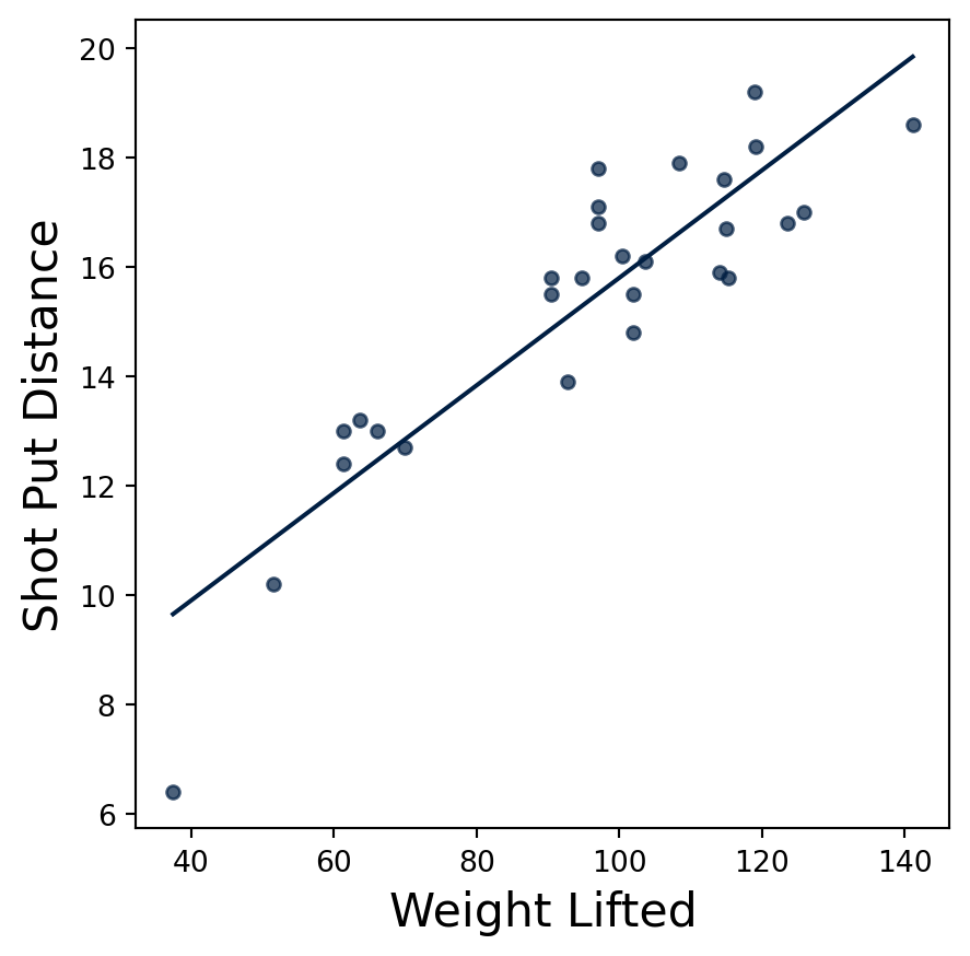
# Generate a scatter plot with `Weight lifted` as the x-axis and `Shot Put Distance` as the y-axisshotput.scatter("Weight Lifted", fit_line=True)plt.show()
Where did that line come from? It is the “line of best fit”, which is the line that minimizes the mean squared error (MSE) between the fitted or predicted values and the actual values. That line is also the “regression line”, i.e, the line that predicts the shot put distance as a function of weight lifted. The different identities for that line give some ideas for how we could compute that line for ourselves:
Determine the regression line
Determine the line of best fit by minimizing mean squared error (MSE)
Using existing library functions for fitting
Regression line
The following describes the slope and intercept for simple linear regression, i.e., a linear regression model with one independent or “explanatory” variable, \(x\), and one dependent variable, \(y\):
where \(\bar{x}\) and \(\bar{y}\) are the means of the \(x\) and \(y\) values, respectively. Let’s implement this calculation as a function regression_line that returns the slope and intercept of the regression line as a numpy array.
We can then apply this function to the shot put data to determine the regression line.
rline = regression_line(shotput["Weight Lifted"], shotput["Shot Put Distance"])rline
array([ 0.09834382, 5.9596291 ])
What does this line imply? That the predicted shot put distance is \(0.098 \times \text{Weight Lifted} + 5.95\). Or alternately, for every additional kilogram the athlete can lift, their shot put personal best dist increases by 0.098 meters.
Where did the slope and intercept come from?
The slope and intercept are derived from the correlation coefficient, \(r\), of the two variables, \(x\) and \(y\). Specifically: \[
\begin{align*}
\text{slope} &= r\cdot \frac{\text{SD of }y}{\text{SD of }x} \\
\text{intercept} &= \bar{y} - \text{slope} \cdot \bar{x}
\end{align*}
\]
The correlation coefficient, \(r\), is a measure of the strength and direction of a linear relationship between two variables. The correlation coefficient ranges from -1 to 1, with 1 indicating a perfect positive linear relationship, -1 indicating a perfect negative linear relationship, and 0 indicating no linear relationship. \(r\) is calculated as the average of the product of the two variables, when they are transformed into standard units. To transform a variable into standard units, we subtract the mean of the variable and divide by the standard deviation. Plugging that into the definition of \(r\) gives:
\[
r = \frac{\sum_{i=1}^{N} \frac{(x_i - \bar{x})}{\text{SD of }x}\frac{(y_i - \bar{y})}{\text{SD of }y}}{N}
\]
We can now express the slope as \[
\begin{align*}
\text{slope} &= r\cdot \frac{\text{SD of }y}{\text{SD of }x} \\
\text{slope} &= \frac{\sum_{i=1}^{N} \frac{(x_i - \bar{x})}{\text{SD of }x}\frac{(y_i - \bar{y})}{\text{SD of }y}}{N} \cdot \frac{\text{SD of }y}{\text{SD of }x} \\
\text{slope} &= \frac{\sum_{i=1}^{N} \frac{(x_i - \bar{x})}{(\text{SD of }x)^2}(y_i - \bar{y})}{N} \\
\text{slope} &= \frac{\sum_{i=1}^{N} \frac{(x_i - \bar{x})N}{\sum_{i=1}^N (x_i - \bar{x})^2}(y_i - \bar{y})}{N} \\
\text{slope} &= \frac{\sum_{i=1}^{N} (x_i - \bar{x})(y_i - \bar{y})}{\sum_{i=1}^{N} (x_i - \bar{x})^2}
\end{align*}
\]
Minimizing mean squared error
We also described the line of best fit as the line that minimizes the mean squared error (MSE) between the fitted values and the actual values. We can perform that minimization by defining a function that calculates the MSE for a given slope and intercept and then using tools in Python’s scientific libraries to find the arguments that minimize the return value of that function. Specifically we can use the minimize function in the datascience library (which is a wrapper around the minimize function in the scipy library).
Let’s start by writing a function fit_mse that takes two parameters, slope and intercept and returns the MSE between the fitted values and the actual values, assuming the input and output data are stored in the variables x and y, respectively. We can then use this function as the argument to the minimize function. minimize will run this function with different values of slope and intercept till it finds the values that minimize the MSE.
We didn’t define where x and y will come from. Wrap your definition of fit_mse in a function mse_line that takes the input data x and y and returns the result of minimize on fit_mse. Doing so creates a nested function that has access to the variables x and y that were defined when the function was created (often called a closure). We have generally discourage the use of nested functions in this course, but they can be useful in certain situations like this one. Here the inputs slope and intercept change during the minimization, while x and y remain fixed. We define the former as the function parameters, and “embed” the latter in the nested function.
def mse_line(x, y):# Create a nested function that takes the parameters to minimize while "closing"# over (embedding) the current x and y values. We can then call this function without# needing to pass x and y as arguments.def fit_mse(slope, intercept): fitted = slope * x + interceptreturn np.mean((y - fitted) **2)# Use the minimize function to find the parameters that minimize the output the# the function passed as an argumentreturn ds.minimize(fit_mse)
We can then apply this function to the shot put data to determine the line that minimizes the MSE. As expected, we get the same slope and intercept as the regression line (within the limits of numerical precision)!
mline = mse_line(shotput["Weight Lifted"], shotput["Shot Put Distance"])mline
array([ 0.09834382, 5.95962911])
How could I use scipy directly?
datascience.minimize provides a convenient wrapper around the scipy.optimize.minimize function that handles initial values, splitting the parameters into separate arguments, etc. We could also use scipy.optimize.minimize directly, with small changes.
Here we define a function scipy_fit_mse that takes the parameters to minimize as an array. We further specify the x and y arrays as additional argument. We will pass those arrays through minimize so we don’t need to create a nested function with those values “embedded” (“closed” over). We then use that function as the argument to minimize, also passing the initial values as the x0 parameters, and a tuple of x and y as the args parameter. minimize will pass the values in the args tuple through as the additional arguments to the function it is minimizing (scipy_fit_mse in this case).
import scipy.optimize as opt# Define a function that takes the parameters to minimize as an array, and the x and y arrays# as additional argumentsdef scipy_fit_mse(params, x, y): fitted = params[0] * x + params[1]return np.mean((y - fitted) **2)def scipy_mse_line(x, y):# Use the minimize function to find the parameters that minimize the output of the function# provided as the first argument. x0 is the initial values. We pass the x and y arrays as a tuple# in the args parameter, which will be passed through to the function as additional arguments (it# becomes the x and y parameters above). result = opt.minimize(scipy_fit_mse, x0=[0, 0], args=(x, y))return result.xscipy_mse_line(shotput["Weight Lifted"], shotput["Shot Put Distance"])
array([ 0.09834371, 5.9596393 ])
Using library functions
We would imagine that fitting a line is a common task, and thus Python’s scientific libraries should already have functions that do this. Indeed, the numpy library has a np.ployfit function that fits a polynomial of a given degree to the data. We can use this function to fit a line to the shot put data.
# Fit a line to the data return parameters as an array, in descending order of degree, e.g.,# [slope, intercept] for a linepline = np.polyfit(shotput["Weight Lifted"], shotput["Shot Put Distance"], 1)pline
array([ 0.09834382, 5.9596291 ])
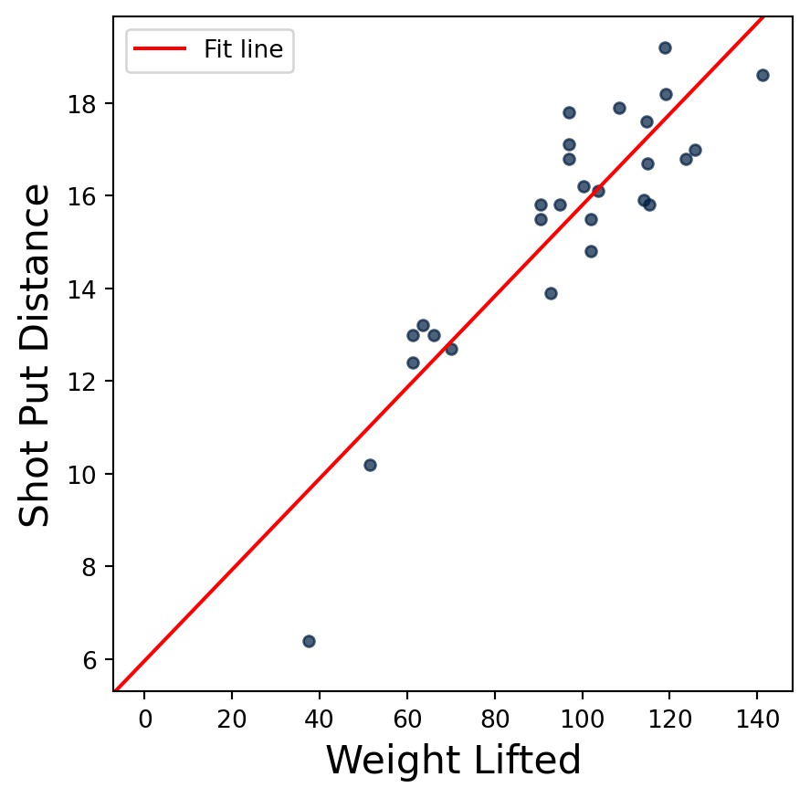
When we apply this function to the shot put data we get the same effective slope and intercept as before (if we didn’t, we would have to check our work). We can then plot this line on top of the scatter plot of the data using the axline function in matplotlib. That function plots an a line given a point and a slope (or two points).
If we look at the title of the source paper, the authors postulate a quadratic relationship between weight lifted and shot put distance. Let’s extend our previous approaches to fit a quadratic function to the data. Recall that the general form of a quadratic function is
\[y = ax^2 + bx + c\]
We can apply a similar approach to finding the quadratic function that minimizes the mean squared error between the fitted values and the actual values. Write a function mse_quadratic that takes the input data x and y and uses minimize to fit a quadratic function to the data. The approach is similar to the linear case, but the implementation for the nested fit_mse function changes.
def mse_quadratic(x, y):# Now fit a quadratic function, i.e., a*x^2 + b*x + c, with 3 parametersdef fit_mse(a, b, c): fitted = a * (x**2) + b * x + creturn np.mean((y - fitted) **2)return ds.minimize(fit_mse)
We can then apply this function to the shot put data. We can also use the np.polyfit function to do the same, increasing the degree of the polynomial to 2 to fit a quadratic function. As expected, we get the same parameters for both approaches (within the limits of numerical precision).
mquad = mse_quadratic(shotput["Weight Lifted"], shotput["Shot Put Distance"])mquad
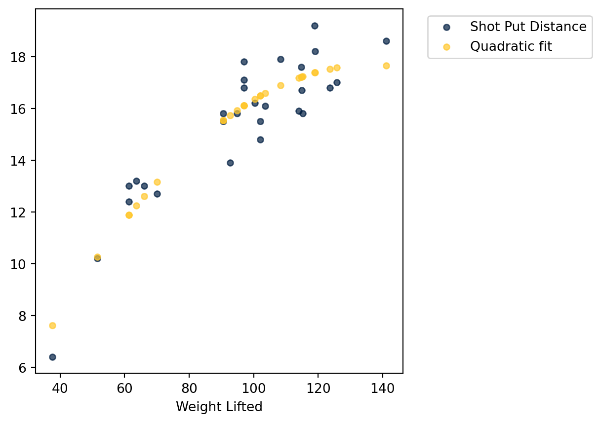
With those fits we can plot the quadratic fit on top of the scatter plot of the data. Here we generate fitted values for the same “x” values as the data and plot those as a second series with the scatter method.
shotput_fit = pquad[0]*(shotput["Weight Lifted"]**2) + pquad[1]*shotput["Weight Lifted"] + pquad[2]# Create a new table with fitted values added as a column, plotting both vs. "Weight lifted"shotput.with_column("Quadratic fit", shotput_fit).scatter("Weight Lifted")plt.show()
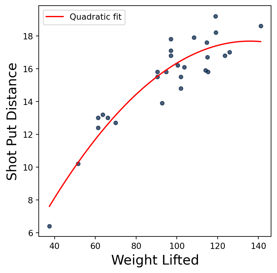
That plot approach makes it difficult to interpolate the fitted values. Instead we would like to plot the fitted curve. Unfortunately there aren’t built functions for plotting quadratic curves just their parameters (as we did the linear line above). Instead we can generate a range of x values and plot the fitted curve over that range as a line plot. Below we use the np.linspace function to generate an array of equally spaced values over the range observed in the data, then compute the expected outputs for those values.
shotput.scatter("Weight Lifted")# Generate "curve" over the range of the data by creating linear spaced "x" values and c# computing the fitted valuesx = np.linspace(shotput["Weight Lifted"].min(), shotput["Weight Lifted"].max(), 100)shotput_fit = pquad[0]*(x**2) + pquad[1]*x + pquad[2]plt.plot(x, shotput_fit, color="red", label="Quadratic fit")plt.legend()plt.show()
Thinking about our data
Our focus here is the computation tools, but that doesn’t mean we shouldn’t think about the data we are working with. Here we fit a quadratic function because it was suggested by the authors of the original study. But if we look at the fit above, it seems that fitted curve is “peaking” and would actually predict shorter distances for even stronger throwers. That is probably not realistic. This suggests that the quadratic model might not be very useful for athletes that are stronger than the ones in the dataset.