Class 19

Data analysis with numpy, datascience and matplotlib: Simulation

Objectives for today

Use the numpy, datascience and matplotlib libraries
Translate iterative code to a vectorized implementation and vice-versa
Implement vectorized simulations

As quick reminder, here are the standard set of imports we are using (note that the order matters, datascience needs to be imported before matplotlib):

import numpy as np
import datascience as ds
import matplotlib
matplotlib.use('TkAgg')
import matplotlib.pyplot as plt

A random walk

A random walk is a path composed of a succession of random steps, e.g. that path of molecule as it travels in a liquid of gas. Random walks have many application in a wide variety of fields from the physical sciences to finance!

A vectorized walk

Let’s start with a very simple 1-D random walk that starts at 0 and takes steps of +1 or -1 with equal probability (source).

How could we implement this walk in a “vectorized” way? What are some capabilities we would need?

Randomly select from 1 and -1 (e.g., similar to random.choice)
Vectorized accumulation

Some relevant NumPy functions: random.choice and cumsum.

Let’s try to write walk_vector function that returns a 1-D NumPy array of the position at each step.

Show an implementation

def walk_vector(steps):
    """ Return array of +1/-1 random walk of length steps """
    # Create random walk by randomly choosing from -1/1
    delta = np.random.choice([-1, 1], steps)
    walk = np.cumsum(delta)
    return walk

An example walk:

walk_vector(100)

array([-1, -2, -3, -2, -3, -2, -3, -4, -3, -2, -3, -4, -3, -4, -3, -2, -3,
       -2, -1,  0,  1,  0,  1,  0, -1,  0,  1,  2,  1,  2,  1,  0,  1,  0,
       -1, -2, -3, -2, -1, -2, -3, -2, -3, -2, -3, -2, -1,  0, -1, -2, -3,
       -4, -3, -2, -1, -2, -3, -2, -1,  0,  1,  0,  1,  0, -1,  0, -1, -2,
       -3, -4, -5, -4, -3, -4, -3, -2, -1,  0,  1,  0,  1,  0, -1, -2, -3,
       -2, -3, -4, -3, -2, -1,  0, -1,  0, -1,  0,  1,  0, -1, -2])

We could plot this walk with Matplotlib as line plot. Let’s try to write a plot_walk function that plots its walk collection parameter such that we can generate the following plot.

Show an implementation

Why don’t we need separate arguments for the “x” and “y” values? The x-values are the step and can entirely be generated from the length of the walk (e.g., with range).

def plot_walk(walk):
    """ Plot random walk as a line plot """
    # We use range to create the "x-axis", i.e., the steps
    plt.plot(range(0, len(walk)), walk)
    plt.xlabel("Step")
    plt.ylabel("Position")
    plt.title("Random walk with +1/-1 steps")
    plt.show()

my_walk = walk_vector(100)
plot_walk(my_walk)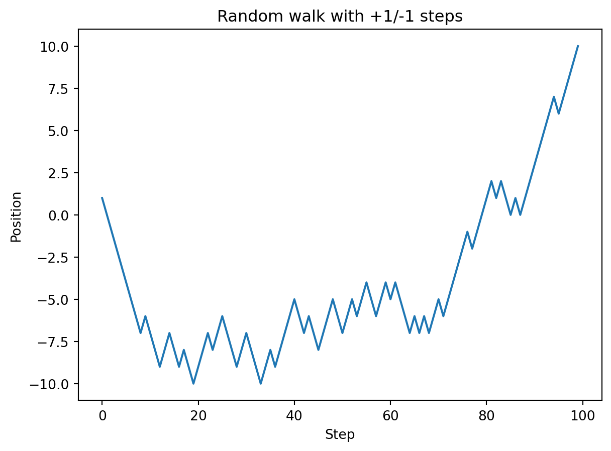

Converting back to “plain” Python

How could we translate this code into a function that just uses Python built-in functions, i.e. doesn’t use NumPy? As starting point we should think about what variables are scalars (i.e. a single value) and which are vectors. The latter would be translated into lists. Operations that produce vectors, translate into loops that build-up lists.

Computing other statistics

We might want to calculate some other statistics, e.g. min and max, and also when the walk reaches its maximum value (i.e the index). For the former we use the NumPy min and max functions so that we use the optimized implementations (instead of the built-in min and max functions).

np.min(my_walk), np.max(my_walk)

(-10, 10)

For determining the index of the maximum, we can use the argmax function. As we discussed earlier, these are large libraries with 100s of functions. Often there is a function “for that”. But no one can or should just know all of these functions. Instead we want to cultivate an idea of what kind of functions should exist and the background/experience to effectively find the relevant function in the documentation.

np.argmax(my_walk)

How would we implement argmax with “built-in” Python?

Scaling it up

Recall that we rarely do a simulation once! Last time for instance we performed 5000 simulations to determine the empirical null distribution for birthweight vs. mother’s smoking status. What if we wanted to compute the maximum values across 5000 random walks? Here is where the vectorized approach can be particularly helpful (for both conciseness and performance). We can think of 5000 random walks of length 100 as working with a 2-D array with 5000 rows and 100 columns. All the NumPy functions we used can also be applied to 2-D (or more than 2-D) arrays!

delta = np.random.choice([-1, 1], (5000, 100))
walks = np.cumsum(delta, axis=1)

Notice we only need to make two changes, one to specify the size as a tuple of length two (rows, columns) and the specify that the cumulative sum should be performed along axis 1, that is along the rows. Here are the resulting walks (note the 2-D array)

walks

array([[-1, -2, -1, ..., 10,  9, 10],
       [ 1,  2,  1, ..., 20, 21, 22],
       [-1, -2, -3, ...,  2,  3,  4],
       ..., 
       [-1,  0,  1, ...,  6,  7,  8],
       [ 1,  0, -1, ...,  4,  5,  4],
       [ 1,  2,  3, ...,  0, -1,  0]])

We can plot the distribution of ending points by selecting the last column in the walks array.

plt.hist(walks[:,-1], bins=30)
plt.xlabel("Final position of walk")
plt.ylabel("Frequency")
plt.show()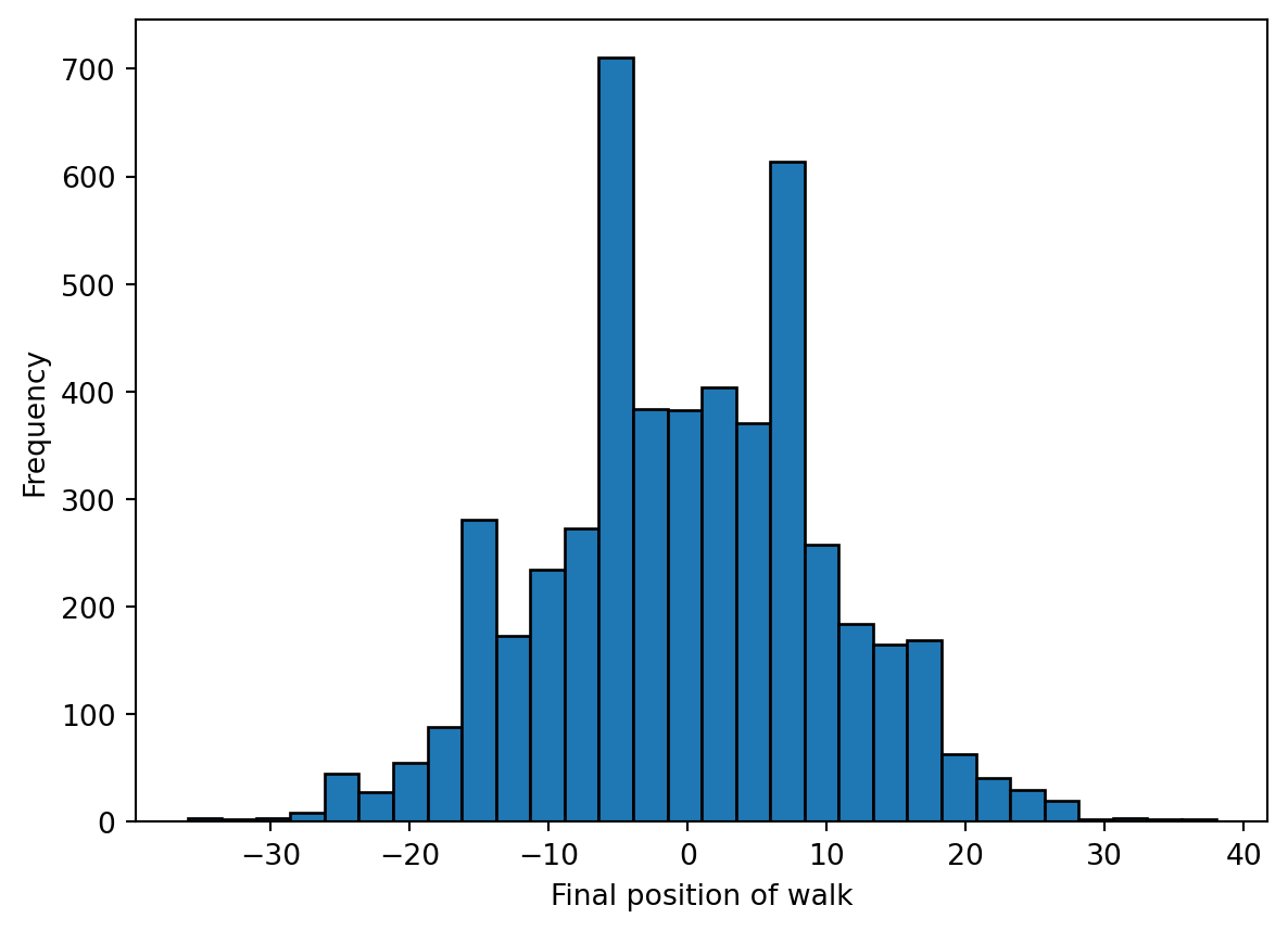

Using random walks

A stock market simulation

We noted earlier that there are many applications for many random walks. One is simulating the stock market (inspiration). A common rule of thumb is that the stock market as a whole will yield 7% a year, but that simplistic model doesn’t capture the variability in returns observed in practice. For example, the S&P 500, a large-cap stock index increased 27% in 2021, but dropped 19.4% in 2022.

An alternate model(Malkiel 2015) (although perhaps not any more accurate) is that that stock market increases 1% per month on average, but with a 4.5 percentage point standard deviation, i.e., on average the market goes up, but there is high variance in those returns. The result could look a lot like the jagged walk we observed earlier![Not investing advice! Our focus here is the implementation. I don’t make any claims about the accuracy of this model. Instead, we exploring how to use the computational tools we are learning about for different purposes.] Let’s try to adapt the approaches we just developed for simulating the stock market.

Malkiel, B. G. 2015. A Random Walk down Wall Street: The Time-Tested Strategy for Successful Investing. Norton.

Let’s assume we start with a portfolio of $100 and simulate 20 years, e.g., 240 months. Each month we observe a random return with a mean of 1% and standard deviation of 4.5% (the random walk). The compounded product of those returns gives our final portfolio amount.

We will need to make some changes from our previous example. There our random walk added or subtracted with uniform probability (i.e., we sampled uniformly from the set of { +1, -1 }). Here we want to sample from a distribution of possible returns (with a mean of 1% and standard deviation of 4.5%). When we sample of from a distribution, we are generating random values with a probability that matches the target distribution. In our case, most samples will be around 1%, with some outliers as described by the standard deviation.

One immediate question is what distribution to use. The probability density function for a Gaussian and Laplace distribution with means of 1.01 (the multiplier for a yield of 1%) and a standard deviation of 4.5% shown below. The details are beyond the scope of our course, but the Laplace distribution offers a better model of the “fat” tails (increased likelihood of outlier events) and asymmetry observed in the stock market. We can use the numpy.random.laplace function to generate random samples from a Laplace distribution. That function is parameterized by the mean and scale (the latter is derived from teh standard deviation).

Code

import math
from scipy.stats import norm, laplace
x = np.linspace(0.6, 1.4, 100)
plt.plot(x, norm.pdf(x, 1.01, 0.045), label="Gaussian")
plt.plot(x, laplace.pdf(x, 1.01, 0.045 / math.sqrt(2)), label="Laplace")
plt.legend()
plt.show()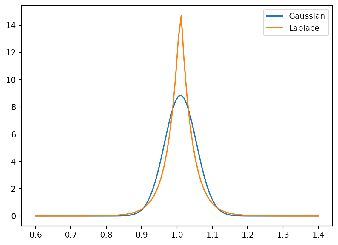

Probability density functions for Gaussian and Laplace distributions

Above our walk was the cumulative sum, here we are interested in the cumulative product of the monthly returns (which we can compute with the cumprod function).

We will start with a single simulation and plot the value of our portfolio at each month:

import math

# Initial portfolio
initial = 100

# Model parameters
mean = 0.01
std = 0.045
scale = std / math.sqrt(2) # Scale parameter for Laplace distribution

# Compute cumulative returns by month
returns = np.cumprod(np.random.laplace(1+mean, scale, 240))
portfolio = initial * returns

plt.plot(range(1, len(portfolio)+1), portfolio)
plt.xlabel("Month")
plt.ylabel("Portfolio ($)")
plt.title("Simulate an investment portfolio of $" + str(initial) + " as a random walk")
plt.show()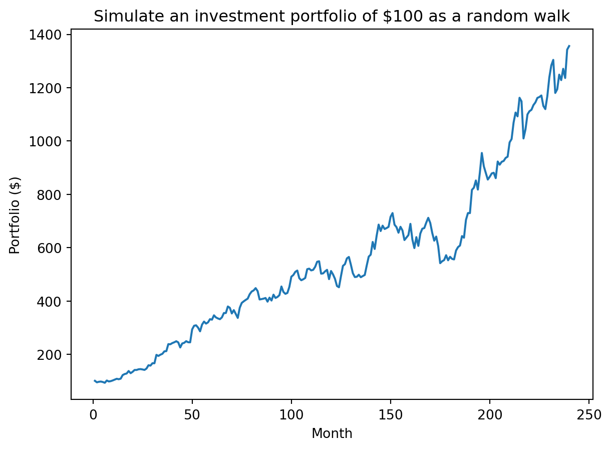

As before we don’t want to do this just once, but many times. We will use a similar technique to generate many walks at once. We can simplify our approach by just focusing on total yield, i.e., compute the product of the returns (with np.prod) not the cumulative product.

num_sim = 5000

# Providing a tuple for size to laplace produces num_simx240 values. We then compute
# the product along axis=1, i.e., along the rows, to get the final return.
returns = np.prod(np.random.laplace(1+mean, scale, (num_sim, 240)), axis=1)
portfolios = initial * returns

We observe a broad distribution of returns

plt.hist(portfolios, bins=30)
plt.xlabel("Portfolio ($)")
plt.ylabel("Frequency")
plt.title("Distribution of portfolios for " + str(num_sim) + " simulations")
plt.show()

including a subset of simulations that underperformed the simplistic model of 7% return per year. Like we did in our previous filtering examples we are performing an element-wise comparison, i.e., comparing each value to initial * average_return, to produce a vector of booleans. When summed, False is treated as 0 and True as 1. Thus the np.sum of the boolean vector calculates the number of Trues.

average_return = 1.07 ** 20
np.sum(portfolios < initial * average_return)

Including continual investment

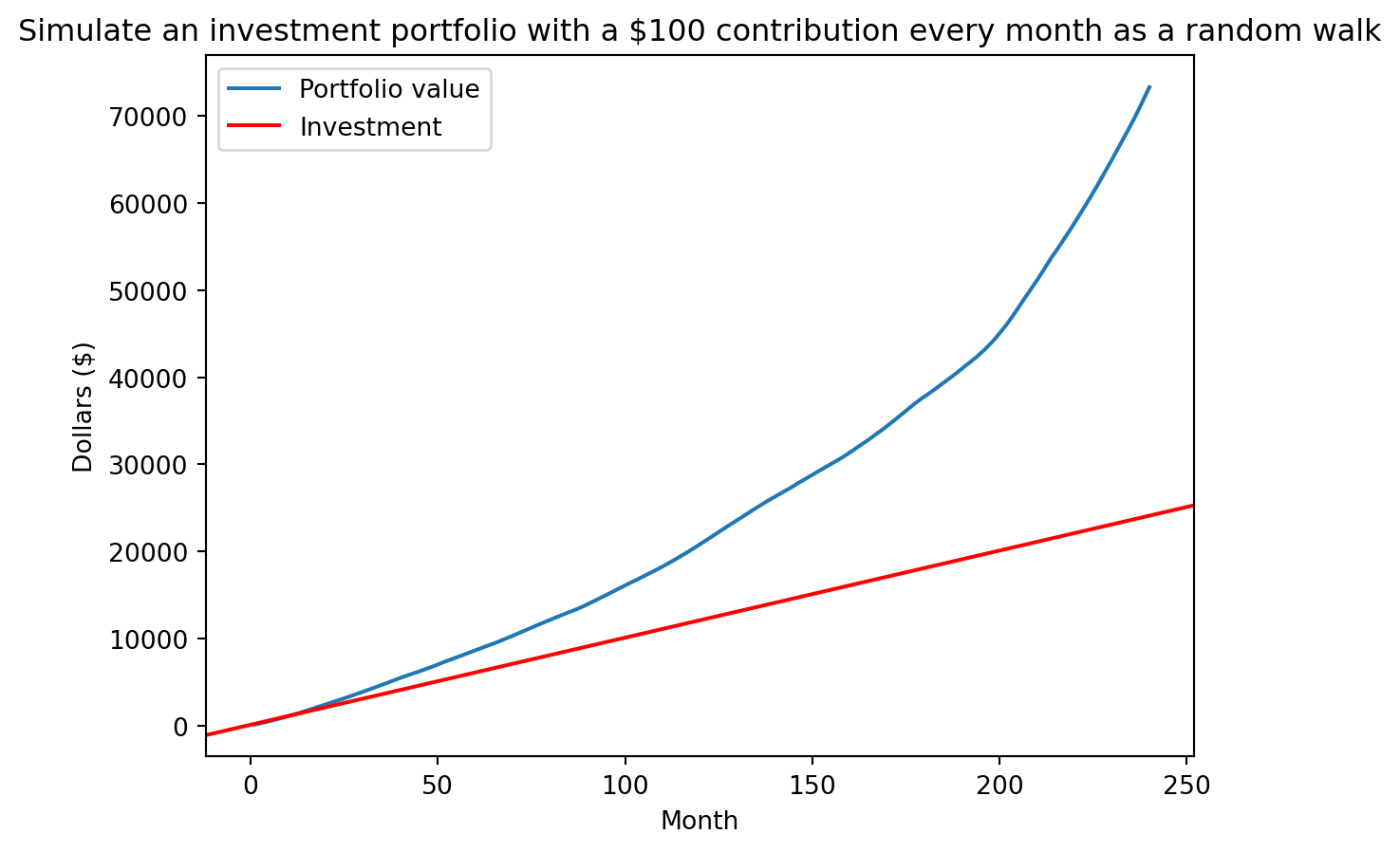
We assumed an initial investment of $100 with no further investments. However a more realistic scenario might be to simulate regular contributions, e.g., contributing a fixed amount each month. How would you extend our previous approach to to model regular contributions? As a suggestion, how can you compute the return on an amount invested for 1 month, 2 months, 3 months … 240 months, and the combine those values to compute the value of the total portfolio? Let’s do so for a single simulation:

# We do exactly the same initial steps as before, but now we think of the returns
# as the total return for each month's investment (albeit in reverse). The first
# entry is the return on the the amount that has been invested for 1 month, the 
# second entry is the return on the amount invested for 2 months, all the way to
# the initial amount invested for 240 months. Now `portfolio` captures final
# amount for each contribution.
returns = np.cumprod(np.random.laplace(1+mean, scale, 240))
portfolio = initial * returns

# Compute the cumulative sum to observe the growth of the portfolio as a whole, 
# i.e., combine the returns for each contribution
portfolio = np.cumsum(portfolio)

We can then plot the value of our portfolio over time (albeit for one simulation):

plt.plot(range(1, len(portfolio)+1), portfolio, label="Portfolio value")
plt.axline((0, initial), slope=initial, color="r", label="Investment")
plt.xlabel("Month")
plt.ylabel("Dollars ($)")
plt.title("Simulate an investment portfolio with a $" + str(initial) + " contribution every month as a random walk")
plt.legend()
plt.show()