Lab 11: Zipf’s Law in R Due: 11:59 PM on 2020-05-11
For this lab we will reimplement the Zipf’s Law lab in R, including both the plotting and printing.
Specification
The specifications are similar to those from lab 10. You will write a program that reads text data from a file and generates the following:
- A printed list of the 10 most frequent words in the file in descending order of frequency along with each word’s count
- A log-log plot of word count versus word rank
Your program must include the following functions:
file_to_wordswhich takes a filename as a parameter and returns a vector of cleaned and normalized words (see below for more details).-
count_and_rankwhich takes a vector of words as a parameter and returns adata.framewithWordandCountcolumns containing the words and their respective counts sorted in descending order of count. For example:> count_and_rank(c("a", "a", "the", "a", "in", "the")) Word Count 1 a 3 3 the 2 2 in 1
When the program starts it should prompt the user to enter the name of a file. Your program should then determine the frequencies of the words in this file, print out the 10 most frequent words, and generate a graph with appropriate data, x-axis and y-axis labels, and title. Your program should only read the file once (to avoid repeating any computations).
Punctuation, e.g., periods or commas, can bias our word counts and so needs to be removed prior to counting. Hyphens and other punctuation within words do not need to be removed. Note that apostrophes in contractions, e.g. “I’ll”, should not be removed (as it would change the word). The starter file contains a function already defined that will strip out leading and trailing punctuation.
Similarly capitalization can bias word counts. Your program should convert all words to lower case to ensure that “The” and “the” are treated as the same word.
Your program should always print the 10 top-ranked words. Your program should also handle the unlikely case that there are fewer than 10 words.
The key difference from your Python implementation is that your R program must not have any explicit loops, i.e. you must exclusively use vector operations.
Creativity points
You may earn up to 2 creativity points on this assignment. Below are some ideas, but you may incorporate your own if you’d like. Make sure to document your additions in comments at the top of the file.
- [0.5 point] Incorporate the filename in the plot title
-
[2 points] Generate the plot using ggplot2. You will want to investigate the
geom_pointfunction, thescale_x_log10andscale_y_log10functions and thelabsfunction. If you invokeggplotfrom your main script RStudio will render the plot (which is OK). If you want to render your plot from within a function, assign the return value fromggplotto a variable andprintthat variable, e.g.plt <- ggplot(...) + ... print(plt)
Example
For the example from “Harry Potter and the Deathly Hallows” (download), your program should produce the following printed output:
 Word Count
  the     8
    a     7
  and     7
   he     7
   to     7
   it     6
  you     6
  but     5
    i     5
   so     5
and the following plots with R base graphics (left) or ggplot2 (right):
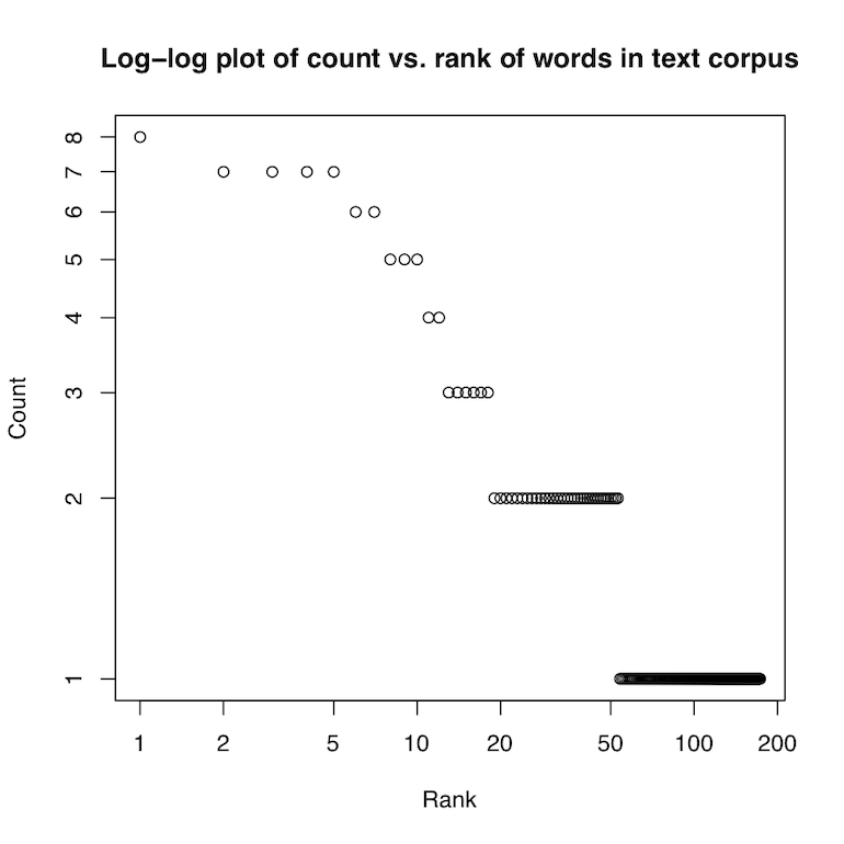
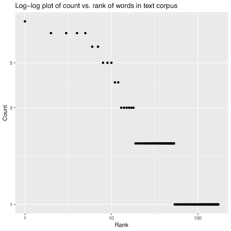
Note that the counts may be slightly different than the Python version due to differences in how the R version handles splitting lines into words and stripping punctuation. Depending on your aesthetic choices for points, etc., your plot might look a little different - that is OK. But the data should be correct and the axis and title labels meaningful.
Guide
We have provided you a starter file that includes several string processing functions mimicking familiar Python methods. Fill in the remaining functions with your code.
Some notes and suggestions
-
You will need to set up the “working directory” in RStudio so it will look for text files in the same directory as your program. (Thonny does that automatically for you.) Open your R program in the RStudio editor and select the RStudio “Session -> Set Working Directory -> To Source File Location” menu option.
- Your first step will be to implement the
file_to_wordsfunction.- You will want to investigate the
readLinesfunction for reading a file into a vector of strings. We suggest settingreadLines’s keyword argumentwarnto beFALSE, e.g.warn=FALSEto eliminate warnings about missing newlines at the end of the file. - The
tolowerfunction is similar to Python’slowermethod.
- You will want to investigate the
-
Incorporate your prelab solution into the
count_and_rankfunction. Note that in some versions of R/RStudio, thecountfunction in plyr is getting overridden by another function with the same name in a different package (but different functionality). To prevent that problem, use the full qualified name, i.e.plyr::count. -
You can sort the rows of a data frame by using the
orderfunction to generate an appropriately ordered list of row indices. Like Python’ssortedfunction,orderhas arguments that will switch the output to descending order. -
Once the rows of your data frame are in sorted order you should be able to generate the ranks where needed with R’s colon operator. Recall that you can access the dimensions of a data frame with the
ncolandnrowfunctions. -
To generate a log-log plot with base graphics, specify the axes to be transformed as a string to the
logkeyword argument toplot, e.g.log="x"for log transformed X-axis,log="y"for a log-transformed Y-axis andlog="xy"to transform both axes. -
To prevent row indices from being printed, you can use the
row.namesoptional keyword argument to the print function, e.g.row.names=FALSE. - The color and fill of the points in your plot don’t have to match examples; it is OK, for instance, to use different colors or solid fill.
Data
Here are several text files you can use for testing, derived from public domain texts at the Project Gutenberg:
-
“Emma” by Jane Austen [local copy as text file] [e-book on Project Gutenberg]
-
“Little Women” by Louisa May Alcott [local copy as text file] [e-book on Project Gutenberg]
-
“David Copperfield” by Charles Dickens [local copy as text file] [e-book on Project Gutenberg]
-
“The Underground Railroad” by William Still [local copy as text file] [e-book on Project Gutenberg]
-
“An Inquiry into the Nature and Causes of the Wealth of Nations” by Adam Smith [local copy as text file] [e-book on Project Gutenberg]
Per the Project Gutenberg license, an eBook is for the use of anyone anywhere at no cost and with almost no restrictions whatsoever. You may copy it, give it away or re-use it under the terms of the Project Gutenberg License included with the eBook or online at www.gutenberg.org.
Start with a smaller test file first – make sure your program is working correctly and efficiently – then tackle a larger dataset. You can also pick interesting inputs of your own from Project Gutenberg or other sources.
When you’re done
Make sure that your program is properly commented:
- You should have comments at the very beginning of the file briefly describing your program and stating your name, section and creativity additions.
- You should have a comment before each function describing the function and its arguments (R does not have formal docstrings like Python).
- Other miscellaneous comments to make things clear
- Remove all ‘# TODO’ comments
In addition, make sure that you’ve used good coding style (including meaningful variable names, constants where relevant, vertical white space, etc.).
Submit your R program via Gradescope. Your program file must be named lab11_zipf_law.R. You can submit multiple times, with only the most recent submission graded. Note that the tests performed by Gradescope are limited. Passing all of the visible tests does not guarantee that your submission correctly satisfies all of the requirements of the assignment.
Grading
| Features | Points |
|---|---|
| Read file and extract words | 3 |
| Word occurrence counts and ranking | 4 |
| Print top 10 words | 3 |
| Plot: Correct data | 4 |
| Plot: Labels, etc. | 2 |
| Code organization | 2 |
| Comments, style | 4 |
| Creativity points | 2 |
| Total | 25 |